General API quickstart

import arviz as az
import matplotlib.pyplot as plt
import numpy as np
import pymc as pm
import pytensor.tensor as pt

/home/xian/anaconda3/envs/pymc-dev-py39/lib/python3.9/site-packages/pkg_resources/__init__.py:123: PkgResourcesDeprecationWarning: main is an invalid version and will not be supported in a future release
  warnings.warn(

RANDOM_SEED = 8927
rng = np.random.default_rng(RANDOM_SEED)
az.style.use("arviz-darkgrid")

1. Model creation

Models in PyMC are centered around the Model class. It has references to all random variables (RVs) and computes the model logp and its gradients. Usually, you would instantiate it as part of a with context:

with pm.Model() as model:
    # Model definition
    pass

We discuss RVs further below but let’s create a simple model to explore the Model class.

with pm.Model() as model:
    mu = pm.Normal("mu", mu=0, sigma=1)
    obs = pm.Normal("obs", mu=mu, sigma=1, observed=rng.standard_normal(100))

model.basic_RVs

[mu ~ N(0, 1), obs ~ N(mu, 1)]

model.free_RVs

[mu ~ N(0, 1)]

model.observed_RVs

[obs ~ N(mu, 1)]

model.compile_logp()({"mu": 0})

array(-143.03962875)

It’s worth highlighting the design choice we made with logp. As you can see above, logp is being called with arguments, so it’s a method of the model instance. More precisely, it puts together a function based on the current state of the model – or on the state given as argument to logp (see example below).

For diverse reasons, we assume that a Model instance isn’t static. If you need to use logp in an inner loop and it needs to be static, simply use something like logp = model.logp. Here is an example below – note the caching effect and the speed up:

%timeit model.compile_logp()({"mu": 0.1})
logp = model.compile_logp()
%timeit logp({"mu": 0.1})

83 ms ± 7.1 ms per loop (mean ± std. dev. of 7 runs, 10 loops each)
18 µs ± 276 ns per loop (mean ± std. dev. of 7 runs, 100,000 loops each)

2. Probability Distributions

Every probabilistic program consists of observed and unobserved Random Variables (RVs). Observed RVs are defined via likelihood distributions, while unobserved RVs are defined via prior distributions. In the PyMC module, the structure for probability distributions looks like this:

Distributions

• pymc:api_distributions_continuous

• pymc:api_distributions_discrete

• pymc:api_distributions_multivariate

• pymc:api_distributions_mixture

• pymc:api_distributions_rimeseries

• pymc:api_distributions_censored

• pymc:api_distributions_simulator

Unobserved Random Variables

Every unobserved RV has the following calling signature: name (str), parameter keyword arguments. Thus, a normal prior can be defined in a model context like this:

with pm.Model():
    x = pm.Normal("x", mu=0, sigma=1)

As with the model, we can evaluate its logp:

pm.logp(x, 0).eval()

array(-0.91893853)

Observed Random Variables

Observed RVs are defined just like unobserved RVs but require data to be passed into the observed keyword argument:

with pm.Model():
    obs = pm.Normal("x", mu=0, sigma=1, observed=rng.standard_normal(100))

observed supports lists, numpy.ndarray and pytensor data structures.

Deterministic transforms

PyMC allows you to freely do algebra with RVs in all kinds of ways:

with pm.Model():
    x = pm.Normal("x", mu=0, sigma=1)
    y = pm.Gamma("y", alpha=1, beta=1)
    plus_2 = x + 2
    summed = x + y
    squared = x**2
    sined = pm.math.sin(x)

Though these transformations work seamlessly, their results are not stored automatically. Thus, if you want to keep track of a transformed variable, you have to use pm.Deterministic:

with pm.Model():
    x = pm.Normal("x", mu=0, sigma=1)
    plus_2 = pm.Deterministic("x plus 2", x + 2)

Note that plus_2 can be used in the identical way to above, we only tell PyMC to keep track of this RV for us.

Lists of RVs / higher-dimensional RVs

Above we have seen how to create scalar RVs. In many models, we want multiple RVs. Users will sometimes try to create lists of RVs, like this:

with pm.Model():
    # bad:
    x = [pm.Normal(f"x_{i}", mu=0, sigma=1) for i in range(10)]

This works, but it is slow and not recommended. Instead, we can use coordinates:

coords = {"cities": ["Santiago", "Mumbai", "Tokyo"]}
with pm.Model(coords=coords) as model:
    # good:
    x = pm.Normal("x", mu=0, sigma=1, dims="cities")

x is now a array of length 3 and each of the 3 variables within this array is associated with a label. This will make it very easy to distinguish the 3 different variables when we go to look at results. We can index into this array or do linear algebra operations on it:

with model:
    y = x[0] * x[1]  # indexing is supported
    x.dot(x.T)  # linear algebra is supported

Initialize Random Variables

Though PyMC automatically initializes models, it is sometimes helpful to define initial values for RVs. This can be done via the initval kwarg:

with pm.Model(coords={"idx": np.arange(5)}) as model:
    x = pm.Normal("x", mu=0, sigma=1, dims="idx")

model.initial_point()

{'x': array([0., 0., 0., 0., 0.])}

with pm.Model(coords={"idx": np.arange(5)}) as model:
    x = pm.Normal("x", mu=0, sigma=1, dims="idx", initval=rng.standard_normal(5))

model.initial_point()

{'x': array([-0.36012097, -0.16168135,  1.07485641, -0.08855632, -0.03857412])}

This technique is sometimes useful when trying to identify problems with model specification or initialization.

3. Inference

Once we have defined our model, we have to perform inference to approximate the posterior distribution. PyMC supports two broad classes of inference: sampling and variational inference.

3.1 Sampling

The main entry point to MCMC sampling algorithms is via the pm.sample() function. By default, this function tries to auto-assign the right sampler(s). pm.sample() returns an arviz.InferenceData object. InferenceData objects can easily be saved/loaded from a file and can carry additional (meta)data such as date/version and posterior predictive samples. Take a look at the ArviZ Quickstart to learn more.

with pm.Model() as model:
    mu = pm.Normal("mu", mu=0, sigma=1)
    obs = pm.Normal("obs", mu=mu, sigma=1, observed=rng.standard_normal(100))

    idata = pm.sample(2000)

Auto-assigning NUTS sampler...
Initializing NUTS using jitter+adapt_diag...
Multiprocess sampling (2 chains in 2 jobs)
NUTS: [mu]

100.00% [6000/6000 00:03<00:00 Sampling 2 chains, 0 divergences]

Sampling 2 chains for 1_000 tune and 2_000 draw iterations (2_000 + 4_000 draws total) took 4 seconds.

As you can see, with model that exclusively contains continuous variables, PyMC assigns the NUTS sampler, which is very efficient even for complex models. PyMC also runs initial tuning to find good starting parameters for the sampler. Here we draw 2000 samples from the posterior in each chain and allow the sampler to adjust its parameters in an additional 1500 iterations.

If not set via the chains kwarg, the number of chains is determined from the number of available CPU cores.

idata.posterior.dims

Frozen({'chain': 2, 'draw': 2000})

The tuning samples are discarded by default. With discard_tuned_samples=False they can be kept and end up in a separate group within the InferenceData object (i.e., idata.warmup_posterior).

You can control how the chains are run in parallel using the chains and cores kwargs:

with pm.Model() as model:
    mu = pm.Normal("mu", mu=0, sigma=1)
    obs = pm.Normal("obs", mu=mu, sigma=1, observed=rng.standard_normal(100))

    idata = pm.sample(cores=4, chains=6)

Auto-assigning NUTS sampler...
Initializing NUTS using jitter+adapt_diag...
Multiprocess sampling (6 chains in 4 jobs)
NUTS: [mu]

100.00% [12000/12000 00:07<00:00 Sampling 6 chains, 0 divergences]

Sampling 6 chains for 1_000 tune and 1_000 draw iterations (6_000 + 6_000 draws total) took 7 seconds.

idata.posterior["mu"].shape

(6, 1000)

# get values of a single chain
idata.posterior["mu"].sel(chain=2).shape

(1000,)

3.2 Analyze sampling results

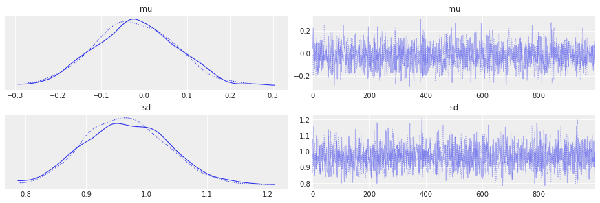
The most common used plot to analyze sampling results is the so-called trace-plot:

with pm.Model() as model:
    mu = pm.Normal("mu", mu=0, sigma=1)
    sd = pm.HalfNormal("sd", sigma=1)
    obs = pm.Normal("obs", mu=mu, sigma=sd, observed=rng.standard_normal(100))

    idata = pm.sample()

Auto-assigning NUTS sampler...
Initializing NUTS using jitter+adapt_diag...
Multiprocess sampling (2 chains in 2 jobs)
NUTS: [mu, sd]

100.00% [4000/4000 00:03<00:00 Sampling 2 chains, 0 divergences]

Sampling 2 chains for 1_000 tune and 1_000 draw iterations (2_000 + 2_000 draws total) took 4 seconds.

az.plot_trace(idata);

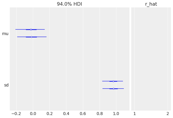
Another common metric to look at is the Gelman-Rubin statistic, or R-hat:

az.summary(idata)

	mean	sd	hdi_3%	hdi_97%	mcse_mean	mcse_sd	ess_bulk	ess_tail	r_hat
mu	-0.019	0.096	-0.193	0.163	0.002	0.002	1608.0	1343.0	1.0
sd	0.967	0.069	0.835	1.089	0.002	0.001	1836.0	1406.0	1.0

R-hat is also presented as part of the az.plot_forest:

az.plot_forest(idata, r_hat=True);

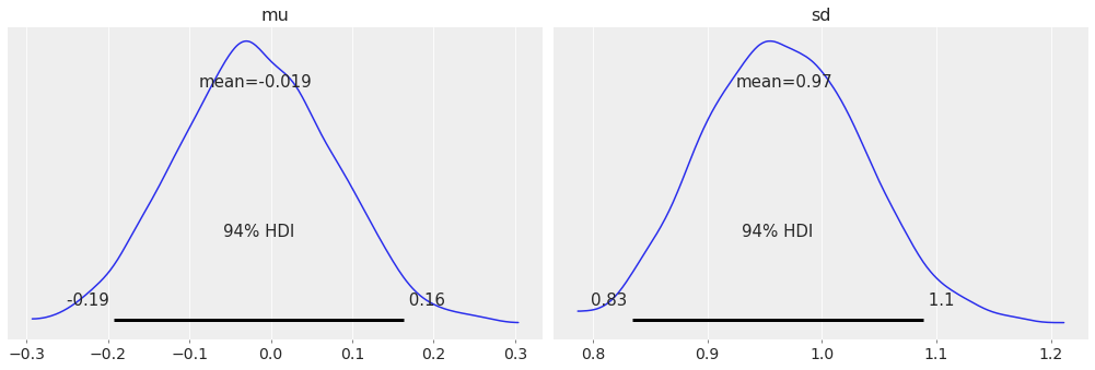
Finally, for a plot of the posterior that is inspired by [Kruschke, 2014], you can use the:

az.plot_posterior(idata);

For high-dimensional models it becomes cumbersome to look at the traces for all parameters. When using NUTS we can look at the energy plot to assess problems of convergence:

with pm.Model(coords={"idx": np.arange(100)}) as model:
    x = pm.Normal("x", mu=0, sigma=1, dims="idx")
    idata = pm.sample()

az.plot_energy(idata);

Auto-assigning NUTS sampler...
Initializing NUTS using jitter+adapt_diag...
Multiprocess sampling (2 chains in 2 jobs)
NUTS: [x]

100.00% [4000/4000 00:04<00:00 Sampling 2 chains, 0 divergences]

Sampling 2 chains for 1_000 tune and 1_000 draw iterations (2_000 + 2_000 draws total) took 5 seconds.

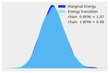
For more information on sampler stats and the energy plot, see Sampler Statistics. For more information on identifying sampling problems and what to do about them, see Diagnosing Biased Inference with Divergences.

3.3 Variational inference

PyMC supports various Variational Inference techniques. While these methods are much faster, they are often also less accurate and can lead to biased inference. The main entry point is pymc.fit().

with pm.Model() as model:
    mu = pm.Normal("mu", mu=0, sigma=1)
    sd = pm.HalfNormal("sd", sigma=1)
    obs = pm.Normal("obs", mu=mu, sigma=sd, observed=rng.standard_normal(100))

    approx = pm.fit()

100.00% [10000/10000 00:00<00:00 Average Loss = 142.01]

Finished [100%]: Average Loss = 142

The returned Approximation object has various capabilities, like drawing samples from the approximated posterior, which we can analyse like a regular sampling run:

idata = approx.sample(1000)
az.summary(idata)

arviz - WARNING - Shape validation failed: input_shape: (1, 1000), minimum_shape: (chains=2, draws=4)

	mean	sd	hdi_3%	hdi_97%	mcse_mean	mcse_sd	ess_bulk	ess_tail	r_hat
mu	-0.023	0.169	-0.338	0.296	0.005	0.004	973.0	880.0	NaN
sd	0.989	0.158	0.694	1.262	0.005	0.004	972.0	1026.0	NaN

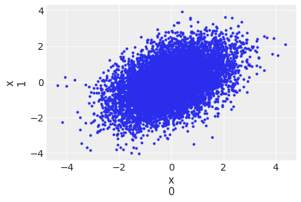
The variational submodule offers a lot of flexibility in which VI to use and follows an object oriented design. For example, full-rank ADVI estimates a full covariance matrix:

mu = pm.floatX([0.0, 0.0])
cov = pm.floatX([[1, 0.5], [0.5, 1.0]])
with pm.Model(coords={"idx": np.arange(2)}) as model:
    pm.MvNormal("x", mu=mu, cov=cov, dims="idx")
    approx = pm.fit(method="fullrank_advi")

100.00% [10000/10000 00:03<00:00 Average Loss = 0.013113]

Finished [100%]: Average Loss = 0.012772

An equivalent expression using the object-oriented interface is:

with pm.Model(coords={"idx": np.arange(2)}) as model:
    pm.MvNormal("x", mu=mu, cov=cov, dims="idx")
    approx = pm.FullRankADVI().fit()

100.00% [10000/10000 00:03<00:00 Average Loss = 0.020591]

Finished [100%]: Average Loss = 0.020531

with pm.Model(coords={"idx": np.arange(2)}) as model:
    pm.MvNormal("x", mu=mu, cov=cov, dims="idx")
    approx = pm.FullRankADVI().fit()

100.00% [10000/10000 00:03<00:00 Average Loss = 0.014234]

Finished [100%]: Average Loss = 0.014143

plt.figure()
idata = approx.sample(10000)
az.plot_pair(idata, var_names="x", coords={"idx": [0, 1]});

<Figure size 432x288 with 0 Axes>

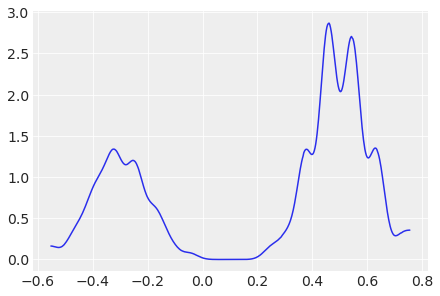
Stein Variational Gradient Descent (SVGD) uses particles to estimate the posterior:

w = pm.floatX([0.2, 0.8])
mu = pm.floatX([-0.3, 0.5])
sd = pm.floatX([0.1, 0.1])
with pm.Model() as model:
    pm.NormalMixture("x", w=w, mu=mu, sigma=sd)
    approx = pm.fit(method=pm.SVGD(n_particles=200, jitter=1.0))

100.00% [10000/10000 01:20<00:00]

with pm.Model() as model:
    pm.NormalMixture("x", w=[0.2, 0.8], mu=[-0.3, 0.5], sigma=[0.1, 0.1])

plt.figure()
idata = approx.sample(10000)
az.plot_dist(idata.posterior["x"]);

For more information on variational inference, see Variational Inference.

4. Posterior Predictive Sampling

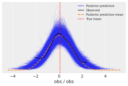
The sample_posterior_predictive() function performs prediction on hold-out data and posterior predictive checks.

data = rng.standard_normal(100)
with pm.Model() as model:
    mu = pm.Normal("mu", mu=0, sigma=1)
    sd = pm.HalfNormal("sd", sigma=1)
    obs = pm.Normal("obs", mu=mu, sigma=sd, observed=data)

    idata = pm.sample()

Auto-assigning NUTS sampler...
Initializing NUTS using jitter+adapt_diag...
Multiprocess sampling (2 chains in 2 jobs)
NUTS: [mu, sd]

100.00% [4000/4000 00:03<00:00 Sampling 2 chains, 0 divergences]

Sampling 2 chains for 1_000 tune and 1_000 draw iterations (2_000 + 2_000 draws total) took 4 seconds.

with model:
    idata.extend(pm.sample_posterior_predictive(idata))

100.00% [2000/2000 00:00<00:00]

fig, ax = plt.subplots()
az.plot_ppc(idata, ax=ax)
ax.axvline(data.mean(), ls="--", color="r", label="True mean")
ax.legend(fontsize=10);

/home/xian/anaconda3/envs/pymc-dev-py39/lib/python3.9/site-packages/IPython/core/pylabtools.py:151: UserWarning: Creating legend with loc="best" can be slow with large amounts of data.
  fig.canvas.print_figure(bytes_io, **kw)

4.1 Predicting on hold-out data

In many cases you want to predict on unseen / hold-out data. This is especially relevant in Probabilistic Machine Learning and Bayesian Deep Learning. PyMC includes a pm.MutableData container to help with such uses. It is a wrapper around a pytensor.shared variable and allows the values of the data to be changed later. Otherwise, pm.MutableData objects can be used just like any other numpy array or tensor.

This distinction is significant since internally all models in PyMC are giant symbolic expressions. When you pass raw data directly into a model, you are giving PyTensor permission to treat this data as a constant and optimize it away if doing so makes sense. If you need to change this data later you may not have any way to point at it within the larger symbolic expression. Using pm.MutableData offers a way to point to a specific place in the symbolic expression and change what is there.

x = rng.standard_normal(100)
y = x > 0

coords = {"idx": np.arange(100)}
with pm.Model() as model:
    # create shared variables that can be changed later on
    x_obs = pm.MutableData("x_obs", x, dims="idx")
    y_obs = pm.MutableData("y_obs", y, dims="idx")

    coeff = pm.Normal("x", mu=0, sigma=1)
    logistic = pm.math.sigmoid(coeff * x_obs)
    pm.Bernoulli("obs", p=logistic, observed=y_obs, dims="idx")
    idata = pm.sample()

Auto-assigning NUTS sampler...
Initializing NUTS using jitter+adapt_diag...
Multiprocess sampling (2 chains in 2 jobs)
NUTS: [x]

100.00% [4000/4000 00:03<00:00 Sampling 2 chains, 0 divergences]

Sampling 2 chains for 1_000 tune and 1_000 draw iterations (2_000 + 2_000 draws total) took 3 seconds.

Now assume we want to predict on unseen data. For this we have to change the values of x_obs and y_obs. Theoretically we don’t need to set y_obs as we want to predict it but it has to match the shape of x_obs.

with model:
    # change the value and shape of the data
    pm.set_data(
        {
            "x_obs": [-1, 0, 1.0],
            # use dummy values with the same shape:
            "y_obs": [0, 0, 0],
        },
        coords={"idx": [1001, 1002, 1003]},
    )

    idata.extend(pm.sample_posterior_predictive(idata))

100.00% [2000/2000 00:00<00:00]

idata.posterior_predictive["obs"].mean(dim=["draw", "chain"])

<xarray.DataArray 'obs' (idx: 3)>
array([0.0215, 0.488 , 0.982 ])
Coordinates:
  * idx      (idx) int64 1001 1002 1003

xarray.DataArray

'obs'

• idx: 3

• 0.0215 0.488 0.982

  array([0.0215, 0.488 , 0.982 ])

• Coordinates: (1)
  • idx
    (idx)
    int64
    1001 1002 1003

    array([1001, 1002, 1003])

• Attributes: (0)

References

[1]

John Kruschke. Doing Bayesian data analysis: A tutorial with R, JAGS, and Stan. Academic Press, 2014.

%load_ext watermark
%watermark -n -u -v -iv -w -p pytensor,aeppl,xarray

Last updated: Fri Jun 03 2022

Python implementation: CPython
Python version       : 3.9.13
IPython version      : 8.4.0

pytensor: 2.6.2
aeppl : 0.0.31
xarray: 2022.3.0

arviz     : 0.12.1
numpy     : 1.22.4
pymc      : 4.0.0b6
pytensor    : 2.6.2
matplotlib: 3.5.2

Watermark: 2.3.1

License notice

All the notebooks in this example gallery are provided under the MIT License which allows modification, and redistribution for any use provided the copyright and license notices are preserved.

Citing PyMC examples

To cite this notebook, use the DOI provided by Zenodo for the pymc-examples repository.

Important

Many notebooks are adapted from other sources: blogs, books… In such cases you should cite the original source as well.

Also remember to cite the relevant libraries used by your code.

Here is an citation template in bibtex:

@incollection{citekey,
  author    = "<notebook authors, see above>",
  title     = "<notebook title>",
  editor    = "PyMC Team",
  booktitle = "PyMC examples",
  doi       = "10.5281/zenodo.5654871"
}

which once rendered could look like: