Bayesian Missing Data Imputation#

import random

import arviz as az
import matplotlib.cm as cm
import matplotlib.pyplot as plt
import numpy as np
import pandas as pd
import pymc as pm
import scipy.optimize

from matplotlib.lines import Line2D
from pymc.sampling.jax import sample_blackjax_nuts, sample_numpyro_nuts
from scipy.stats import multivariate_normal

/Users/nathanielforde/opt/miniconda3/envs/missing_data_clean/lib/python3.11/site-packages/pymc/sampling/jax.py:39: UserWarning: This module is experimental.
  warnings.warn("This module is experimental.")

Bayesian Imputation and Degrees of Missing-ness#

The analysis of data with missing values is a gateway into the study of causal inference.

One of the key features of any analysis plagued by missing data is the assumption which governs the nature of the missing-ness i.e. what is the reason for gaps in our data? Can we ignore them? Should we worry about why? In this notebook we’ll see an example of how to handle missing data using maximum likelihood estimation and bayesian imputation techniques. This will open up questions about the assumptions governing inference in the presence of missing data, and inference in counterfactual cases.

We will make the discussion concrete by considering an example analysis of an employee satisfaction survey and how different work conditions contribute to the responses and non-responses we see in the data.

%config InlineBackend.figure_format = 'retina'  # high resolution figures
az.style.use("arviz-darkgrid")
rng = np.random.default_rng(42)

Missing Data Taxonomy#

Rubin’s famous taxonomy breaks out the question into a choice of three fundamental options:

Missing Completely at Random (MCAR)
Missing at Random (MAR)
Missing Not at Random (MNAR)

Each of these paradigms can be reduced to explicit definition in terms of the conditional probability regarding the pattern of missing data. The first pattern is the least concerning. The (MCAR) assumption states that the data are missing in a manner that is unrelated to both the observed and unobserved parts of the realised data. It is missing due to the haphazard circumstance of the world \(\phi\).

\[ P(M =1 | Y_{obs}, Y_{miss}, \phi) = P(M =1 | \phi) \]

whereas the second pattern (MAR) allows that the reasons for missingness can be function of the observed data and circumstances of the world. Some times this is called a case of ignorable missingness because estimation can proceed in good faith on the basis of the observed data. There may be a loss of precision, but the inference should be sound.

\[ P(M =1 | Y_{obs}, Y_{miss}, \phi) = P(M =1 | Y_{obs}, \phi) \]

The most nefarious sort of missing data is when the missingness is a function of something outside the observed data, and the equation cannot be reduced further. Efforts at imputation and estimation more generally may become more difficulty in this final case because of the risk of confounding. This is a case of non-ignorable missing-ness.

\[ P(M =1 | Y_{obs}, Y_{miss}, \phi) \]

These assumptions are made before any analysis begins. They are inherently unverifiable. Your analysis will stand or fall depending on how plausible each assumption is in the context you seek to apply them. For example, an another type missing data results from systematic censoring as discussed in Bayesian regression with truncated or censored data. In such cases the reason for censoring governs the missing-ness pattern.

Employee Satisfaction Surveys#

We’ll follow the presentation of Craig Enders’ Applied Missing Data Analysis Enders K [2022] and work with employee satisifaction data set. The data set comprises of a few composite measures reporting employee working conditions and satisfactions. Of particular note are empowerment (empower), work satisfaction (worksat) and two composite survey scores recording the employees leadership climate (climate), and the relationship quality with their supervisor lmx.

The key question is what assumptions governs our patterns of missing data.

try:
    df_employee = pd.read_csv("../data/employee.csv")
except FileNotFoundError:
    df_employee = pd.read_csv(pm.get_data("employee.csv"))
df_employee.head()

	employee	team	turnover	male	empower	lmx	worksat	climate	cohesion
0	1	1	0.0	1	32.0	11.0	3.0	18.0	3.5
1	2	1	1.0	1	NaN	13.0	4.0	18.0	3.5
2	3	1	1.0	1	30.0	9.0	4.0	18.0	3.5
3	4	1	1.0	1	29.0	8.0	3.0	18.0	3.5
4	5	1	1.0	0	26.0	7.0	4.0	18.0	3.5

# Percentage Missing
df_employee[["worksat", "empower", "lmx"]].isna().sum() / len(df_employee)

worksat    0.047619
empower    0.161905
lmx        0.041270
dtype: float64

# Patterns of missing Data
df_employee[["worksat", "empower", "lmx"]].isnull().drop_duplicates().reset_index(drop=True)

	worksat	empower	lmx
0	False	False	False
1	False	True	False
2	True	True	False
3	False	False	True
4	True	False	False

fig, ax = plt.subplots(figsize=(20, 7))
ax.hist(df_employee["empower"], bins=30, ec="black", color="cyan", label="Empowerment")
ax.hist(df_employee["lmx"], bins=30, ec="black", color="yellow", label="LMX")
ax.hist(df_employee["worksat"], bins=30, ec="black", color="green", label="Work Satisfaction")
ax.set_title("Employee Satisfaction Survey Results", fontsize=20)
ax.legend();

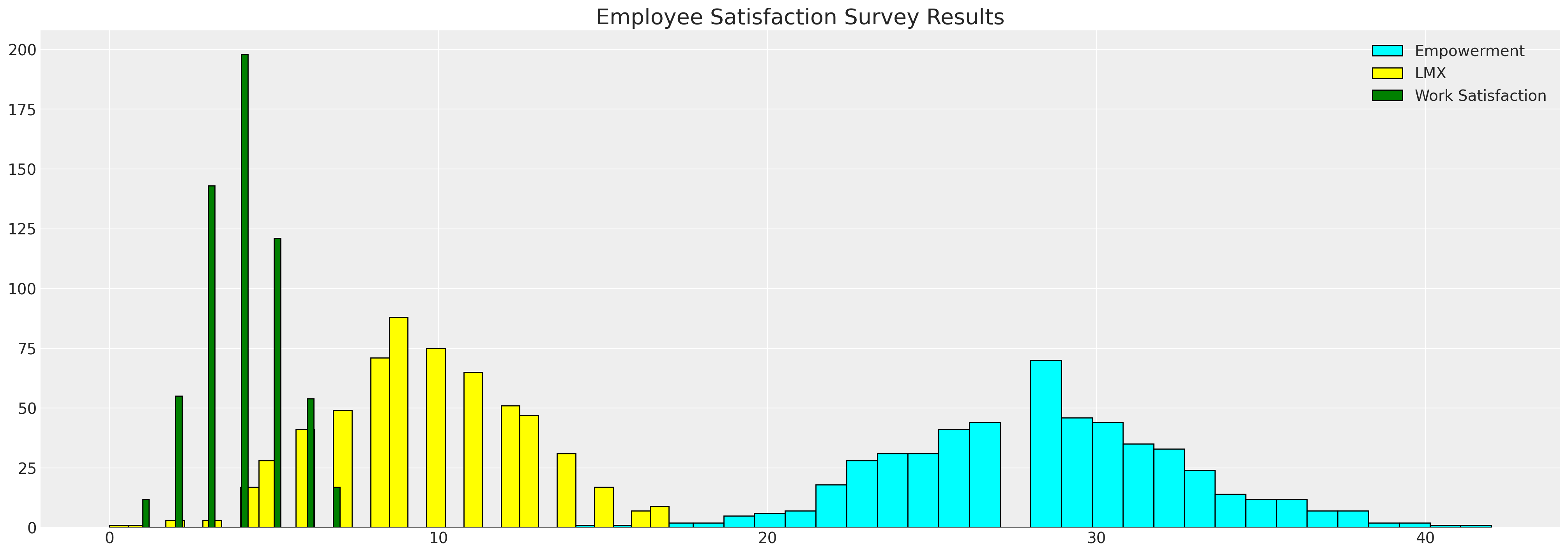
../_images/4651aee3b14cc8fcb4f416403736e3ecb5f7f8ce1171367a38f6c44a02888f86.png

We see here the histograms of the employee metrics. It is the gaps in the data that we wish to impute to better understand the relationships between the variables and how gaps in one may be driven by values in the others.

FIML: Full Information Maximum Likelihood#

This method of handling missing data is not an imputation method. It uses maximum likelihood estimation to estimate the parameters of the multivariate normal distribution that could be best said to generate our observed data. It’s a little trickier than straight forward MLE approaches in that it respects the fact that we have missing data in our original data set, but fundamentally it’s the same idea. We want to optimize the parameters of our multivariate normal distribution to best fit the observed data.

The procedure works by partitioning the data into their patterns of “missing-ness” and treating each partition as contributing to the ultimate log-likelihood term that we want to maximise. We combine their contributions to estimate a fit for the multivariate normal distribution.

data = df_employee[["worksat", "empower", "lmx"]]


def split_data_by_missing_pattern(data):
    # We want to extract our the pattern of missing-ness in our dataset
    # and save each sub-set of our data in a structure that can be used to feed into a log-likelihood function
    grouped_patterns = []
    patterns = data.notnull().drop_duplicates().values
    # A pattern is whether the values in each column e.g. [True, True, True] or [True, True, False]
    observed = data.notnull()
    for p in range(len(patterns)):
        temp = observed[
            (observed["worksat"] == patterns[p][0])
            & (observed["empower"] == patterns[p][1])
            & (observed["lmx"] == patterns[p][2])
        ]
        grouped_patterns.append([patterns[p], temp.index, data.iloc[temp.index].dropna(axis=1)])

    return grouped_patterns


def reconstitute_params(params_vector, n_vars):
    # Convenience numpy function to construct mirrored COV matrix
    # From flattened params_vector
    mus = params_vector[0:n_vars]
    cov_flat = params_vector[n_vars:]
    indices = np.tril_indices(n_vars)
    cov = np.empty((n_vars, n_vars))
    for i, j, c in zip(indices[0], indices[1], cov_flat):
        cov[i, j] = c
        cov[j, i] = c
    cov = cov + 1e-25
    return mus, cov


def optimise_ll(flat_params, n_vars, grouped_patterns):
    mus, cov = reconstitute_params(flat_params, n_vars)
    # Check if COV is positive definite
    if (np.linalg.eigvalsh(cov) < 0).any():
        return 1e100
    objval = 0.0
    for obs_pattern, _, obs_data in grouped_patterns:
        # This is the key (tricky) step because we're selecting the variables which pattern
        # the full information set within each pattern of "missing-ness"
        # e.g. when the observed pattern is [True, True, False] we want the first two variables
        # of the mus vector and we want only the covariance relations between the relevant variables from the cov
        # in the iteration.
        obs_mus = mus[obs_pattern]
        obs_cov = cov[obs_pattern][:, obs_pattern]
        ll = np.sum(multivariate_normal(obs_mus, obs_cov).logpdf(obs_data))
        objval = ll + objval
    return -objval


def estimate(data):
    n_vars = data.shape[1]
    # Initialise
    mus0 = np.zeros(n_vars)
    cov0 = np.eye(n_vars)
    # Flatten params for optimiser
    params0 = np.append(mus0, cov0[np.tril_indices(n_vars)])
    # Process Data
    grouped_patterns = split_data_by_missing_pattern(data)
    # Run the Optimiser.
    try:
        result = scipy.optimize.minimize(
            optimise_ll, params0, args=(n_vars, grouped_patterns), method="Powell"
        )
    except Exception as e:
        raise e
    mean, cov = reconstitute_params(result.x, n_vars)
    return mean, cov


fiml_mus, fiml_cov = estimate(data)


print("Full information Maximum Likelihood Estimate Mu:")
display(pd.DataFrame(fiml_mus, index=data.columns).T)
print("Full information Maximum Likelihood Estimate COV:")
pd.DataFrame(fiml_cov, columns=data.columns, index=data.columns)

Full information Maximum Likelihood Estimate Mu:

	worksat	empower	lmx
0	3.983351	28.595211	9.624485

Full information Maximum Likelihood Estimate COV:

	worksat	empower	lmx
worksat	1.568676	1.599817	1.547433
empower	1.599817	19.138522	5.428954
lmx	1.547433	5.428954	8.934030

Sampling from the Implied Distribution#

We can then sample from the implied distribution to estimate other features of interest and test against the observed data.

mle_fit = multivariate_normal(fiml_mus, fiml_cov)
mle_sample = mle_fit.rvs(10000)
mle_sample = pd.DataFrame(mle_sample, columns=["worksat", "empower", "lmx"])
mle_sample.head()

	worksat	empower	lmx
0	4.467296	31.568011	12.418765
1	4.713191	30.329419	10.651786
2	5.699765	35.770312	12.558135
3	4.067691	27.874578	6.271341
4	3.580109	28.799105	9.704713

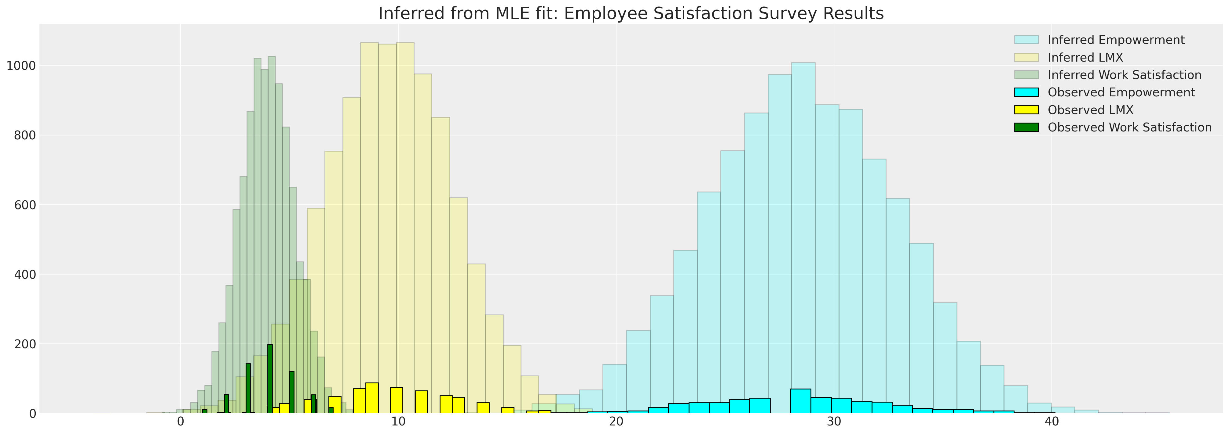
This allows us to compare the implied distributions against the observed data

fig, ax = plt.subplots(figsize=(20, 7))
ax.hist(
    mle_sample["empower"],
    bins=30,
    ec="black",
    color="cyan",
    alpha=0.2,
    label="Inferred Empowerment",
)
ax.hist(mle_sample["lmx"], bins=30, ec="black", color="yellow", alpha=0.2, label="Inferred LMX")
ax.hist(
    mle_sample["worksat"],
    bins=30,
    ec="black",
    color="green",
    alpha=0.2,
    label="Inferred Work Satisfaction",
)
ax.hist(data["empower"], bins=30, ec="black", color="cyan", label="Observed Empowerment")
ax.hist(data["lmx"], bins=30, ec="black", color="yellow", label="Observed LMX")
ax.hist(data["worksat"], bins=30, ec="black", color="green", label="Observed Work Satisfaction")
ax.set_title("Inferred from MLE fit: Employee Satisfaction Survey Results", fontsize=20)
ax.legend()

<matplotlib.legend.Legend at 0x1914bce50>

../_images/c9989dd8511d1b594a2a82b778f8eea3617da7df1135c6bd3dd174a50acb4e2e.png

The Correlation Between the Imputed Metrics Data#

We can also calculate other features of interest from our sample. For instance, we might want to know about the correlations between variables in question.

pd.DataFrame(mle_sample.corr(), columns=data.columns, index=data.columns)

	worksat	empower	lmx
worksat	1.000000	0.300790	0.409996
empower	0.300790	1.000000	0.410874
lmx	0.409996	0.410874	1.000000

Bootstrapping Sensitivity Analysis#

We may also want to validate the estimated parameters against bootstrapped samples under different speficiations of missing-ness.

data_200 = df_employee[["worksat", "empower", "lmx"]].dropna().sample(200)
data_200.reset_index(inplace=True, drop=True)


sensitivity = {}
n_missing = np.linspace(30, 100, 5)  # Change or alter the range as desired
bootstrap_iterations = 100  # change to large number running a real analysis in this case
for n in n_missing:
    sensitivity[int(n)] = {}
    sensitivity[int(n)]["mus"] = []
    sensitivity[int(n)]["cov"] = []
    for i in range(bootstrap_iterations):
        temp = data_200.copy()
        for m in range(int(n)):
            i = random.choice(range(200))
            j = random.choice(range(3))
            temp.iloc[i, j] = np.nan
        try:
            fiml_mus, fiml_cov = estimate(temp)
            sensitivity[int(n)]["mus"].append(fiml_mus)
            sensitivity[int(n)]["cov"].append(fiml_cov)
        except Exception as e:
            next

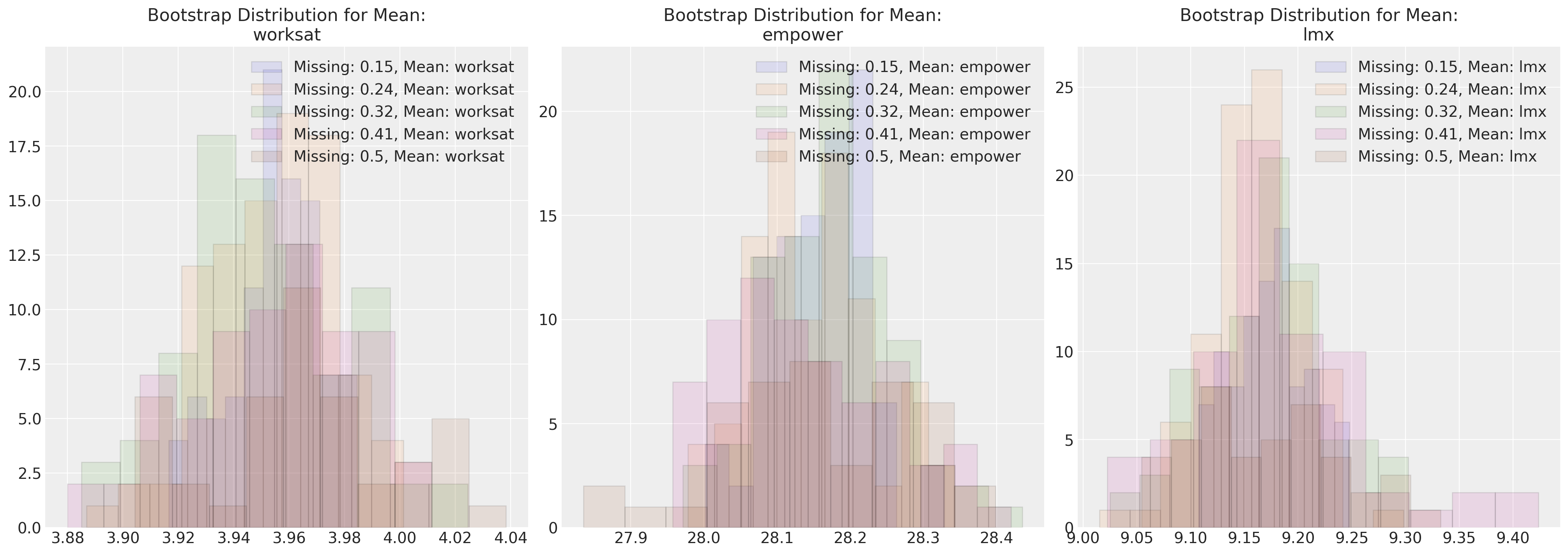
Here we plot the maximum likelihood parameter estimates against various missing data regimes. This approach can be applied for any imputation methodology.

fig, axs = plt.subplots(1, 3, figsize=(20, 7))
for n in sensitivity.keys():
    temp = pd.DataFrame(sensitivity[n]["mus"], columns=["worksat", "empower", "lmx"])
    for col, ax in zip(temp.columns, axs):
        ax.hist(
            temp[col], alpha=0.1, ec="black", label=f"Missing: {np.round(n/200, 2)}, Mean: {col}"
        )
        ax.legend()
        ax.set_title(f"Bootstrap Distribution for Mean:\n{col}")

../_images/d406761320e44acea544dbea124c07552ca5f75f8abf7aeb3e2b766584634412.png

fig, axs = plt.subplots(2, 3, figsize=(20, 14))
axs = axs.flatten()
for n in sensitivity.keys():
    length = len(sensitivity[n]["cov"])
    temp = pd.DataFrame(
        [sensitivity[n]["cov"][i][np.tril_indices(3)] for i in range(length)],
        columns=[
            "var(worksat)",
            "cov(worksat, empower)",
            "var(empower)",
            "cov(worksat, lmx)",
            "cov(lmx, empower)",
            "var(lmx)",
        ],
    )
    for col, ax in zip(temp.columns, axs):
        ax.hist(
            temp[col], alpha=0.1, ec="black", label=f"Missing: {np.round(n/200, 2)}, Mean: {col}"
        )
        ax.legend()
        ax.set_title(f"Bootstrap Distribution for Expected:\n{col}")

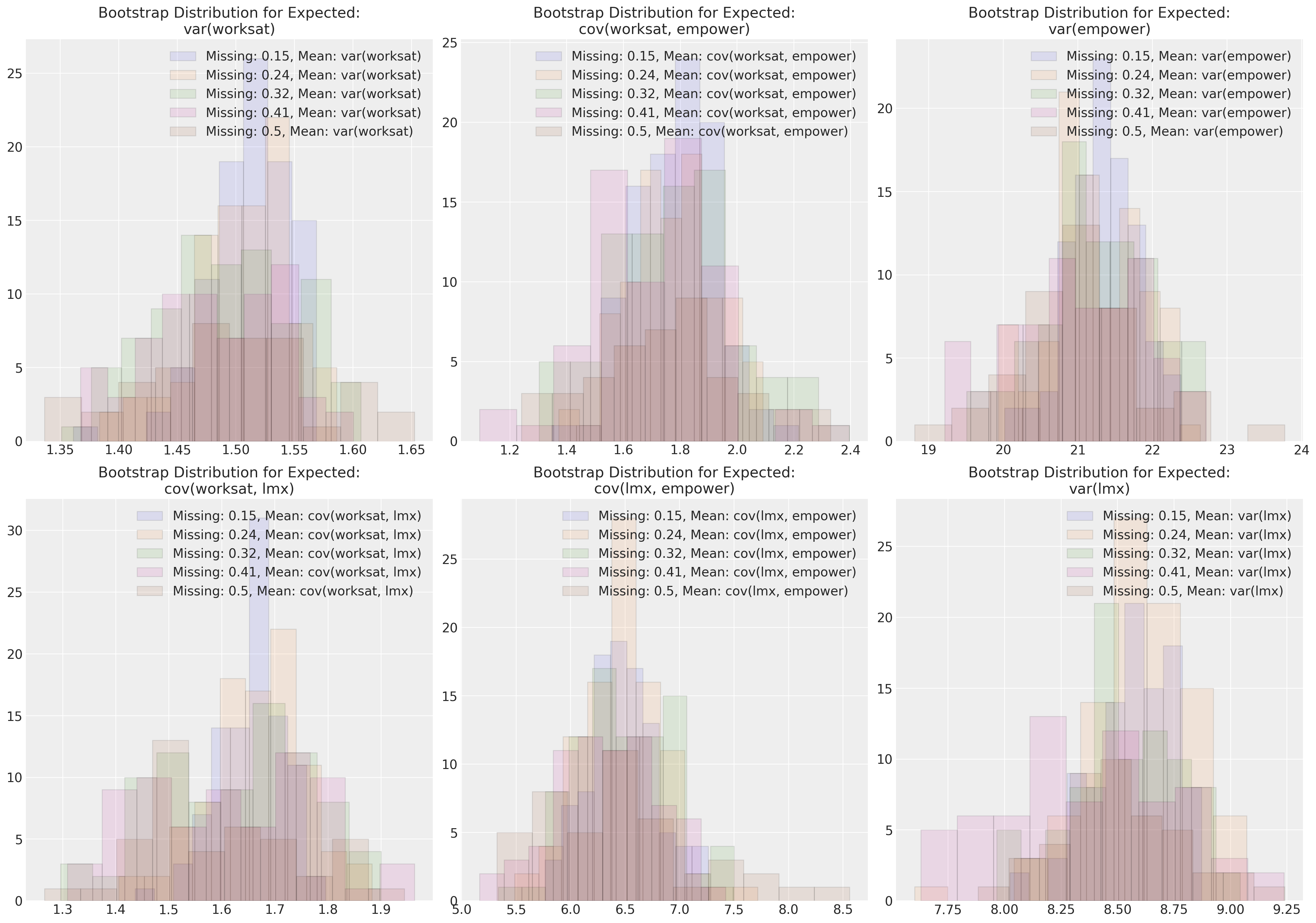
../_images/ae88dc8b4d03fb9c8f319ed9d20c3eaece6a5086508253abfb364412aad42e66.png

These plots show how under (MCAR) the parameter estimates of our multivariate normal distribution are quite robust to varying degrees of missing data. It’s an instructive exercise to attempt a similar simulation exercise under alternative missing data regimes.

Bayesian Imputation#

Next we’ll apply bayesian methods to the same problem. But here we’ll see direct imputation of the missing values using the posterior predictive distribution. The Bayesian approach to imputation is of a different flavour than we saw above. We’re not just learning parameters of the data generating distribution (although we are doing that too), the bayesian process directly imputes the missing values for specific missing entries through the process of MCMC sampling.

import pytensor.tensor as pt

with pm.Model() as model:
    # Priors
    mus = pm.Normal("mus", 0, 1, size=3)
    cov_flat_prior, _, _ = pm.LKJCholeskyCov("cov", n=3, eta=1.0, sd_dist=pm.Exponential.dist(1))
    # Create a vector of flat variables for the unobserved components of the MvNormal
    x_unobs = pm.Uniform("x_unobs", 0, 100, shape=(np.isnan(data.values).sum(),))

    # Create the symbolic value of x, combining observed data and unobserved variables
    x = pt.as_tensor(data.values)
    x = pm.Deterministic("x", pt.set_subtensor(x[np.isnan(data.values)], x_unobs))

    # Add a Potential with the logp of the variable conditioned on `x`
    pm.Potential("x_logp", pm.logp(rv=pm.MvNormal.dist(mus, chol=cov_flat_prior), value=x))
    idata = pm.sample_prior_predictive()
    idata = pm.sample()
    idata.extend(pm.sample(random_seed=120))
    pm.sample_posterior_predictive(idata, extend_inferencedata=True)

pm.model_to_graphviz(model)

/var/folders/99/gp2xl6x513s0tvl3cx79zf7m0000gn/T/ipykernel_96943/3865616598.py:16: UserWarning: The effect of Potentials on other parameters is ignored during prior predictive sampling. This is likely to lead to invalid or biased predictive samples.
  idata = pm.sample_prior_predictive()
Sampling: [cov, mus, x_unobs]
Auto-assigning NUTS sampler...
Initializing NUTS using jitter+adapt_diag...
Multiprocess sampling (4 chains in 4 jobs)
NUTS: [mus, cov, x_unobs]

100.00% [8000/8000 01:07<00:00 Sampling 4 chains, 0 divergences]

/Users/nathanielforde/opt/miniconda3/envs/missing_data_clean/lib/python3.11/site-packages/pytensor/compile/function/types.py:972: RuntimeWarning: invalid value encountered in accumulate
  self.vm()
Sampling 4 chains for 1_000 tune and 1_000 draw iterations (4_000 + 4_000 draws total) took 98 seconds.
Auto-assigning NUTS sampler...
Initializing NUTS using jitter+adapt_diag...
Multiprocess sampling (4 chains in 4 jobs)
NUTS: [mus, cov, x_unobs]

100.00% [8000/8000 01:06<00:00 Sampling 4 chains, 0 divergences]

/Users/nathanielforde/opt/miniconda3/envs/missing_data_clean/lib/python3.11/site-packages/pytensor/compile/function/types.py:972: RuntimeWarning: invalid value encountered in accumulate
  self.vm()
/Users/nathanielforde/opt/miniconda3/envs/missing_data_clean/lib/python3.11/site-packages/pytensor/compile/function/types.py:972: RuntimeWarning: invalid value encountered in accumulate
  self.vm()
Sampling 4 chains for 1_000 tune and 1_000 draw iterations (4_000 + 4_000 draws total) took 99 seconds.
/var/folders/99/gp2xl6x513s0tvl3cx79zf7m0000gn/T/ipykernel_96943/3865616598.py:19: UserWarning: The effect of Potentials on other parameters is ignored during posterior predictive sampling. This is likely to lead to invalid or biased predictive samples.
  pm.sample_posterior_predictive(idata, extend_inferencedata=True)

../_images/f5edcd5cd53a6b22f7ffa3c6ce7dc02ec1405b582c264ced467a302ce2b9d71b.svg

az.plot_posterior(idata, var_names=["mus", "cov"]);

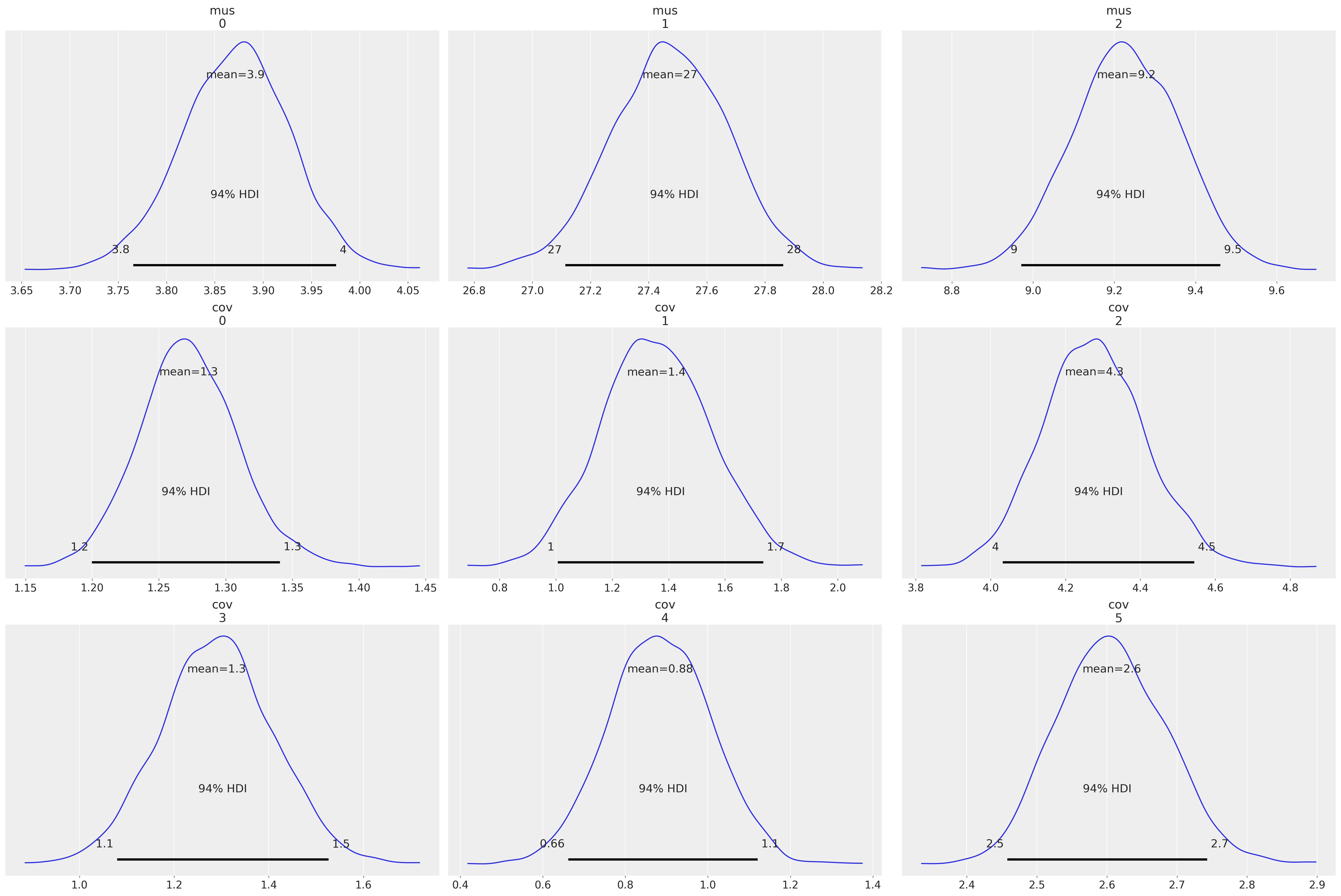
../_images/80dabbe534791f369229f0d2c183e00181aa6debc971e677e68505f3a1e21519.png

az.summary(idata, var_names=["mus", "cov", "x_unobs"])

	mean	sd	hdi_3%	hdi_97%	mcse_mean	mcse_sd	ess_bulk	ess_tail	r_hat
mus[0]	3.871	0.056	3.766	3.976	0.001	0.001	6110.0	3277.0	1.0
mus[1]	27.473	0.200	27.114	27.863	0.003	0.002	5742.0	3320.0	1.0
mus[2]	9.229	0.132	8.971	9.461	0.002	0.001	6154.0	3271.0	1.0
cov[0]	1.272	0.037	1.200	1.341	0.000	0.000	6235.0	2754.0	1.0
cov[1]	1.356	0.197	1.007	1.736	0.003	0.002	5373.0	3750.0	1.0
...	...	...	...	...	...	...	...	...	...
x_unobs[153]	29.836	4.205	21.820	37.745	0.044	0.031	9232.0	2929.0	1.0
x_unobs[154]	2.559	1.107	0.356	4.483	0.018	0.013	3564.0	1634.0	1.0
x_unobs[155]	30.071	4.029	22.614	37.652	0.039	0.028	10697.0	3078.0	1.0
x_unobs[156]	29.654	4.017	22.079	37.411	0.039	0.027	10626.0	2867.0	1.0
x_unobs[157]	27.420	4.066	19.595	34.915	0.046	0.033	7784.0	2226.0	1.0

167 rows × 9 columns

imputed_dims = data.shape
imputed = data.values.flatten()
imputed[np.isnan(imputed)] = az.summary(idata, var_names=["x_unobs"])["mean"].values
imputed = imputed.reshape(imputed_dims[0], imputed_dims[1])
imputed = pd.DataFrame(imputed, columns=[col + "_imputed" for col in data.columns])
imputed.head(10)

	worksat_imputed	empower_imputed	lmx_imputed
0	3.000	32.000	11.000
1	4.000	29.431	13.000
2	4.000	30.000	9.000
3	3.000	29.000	8.000
4	4.000	26.000	7.000
5	3.995	27.915	10.000
6	5.000	28.984	11.000
7	3.000	22.000	9.000
8	2.000	23.000	6.835
9	4.000	32.000	9.000

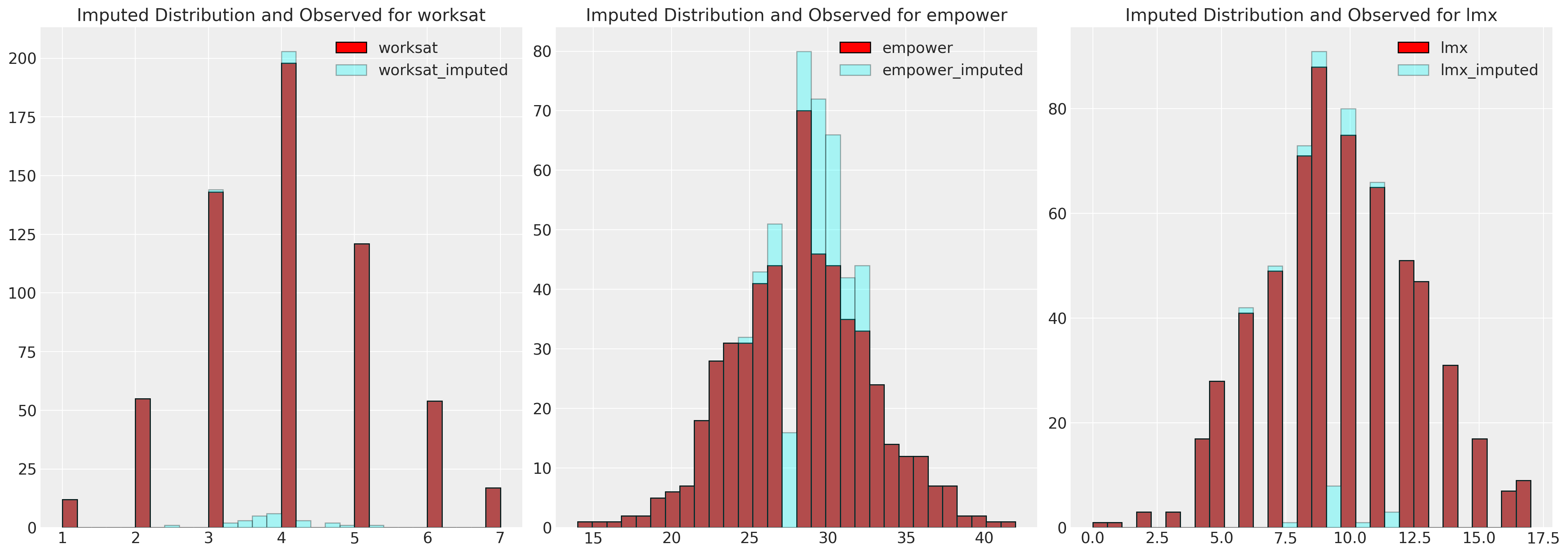
fig, axs = plt.subplots(1, 3, figsize=(20, 7))
axs = axs.flatten()
for col, col_i, ax in zip(data.columns, imputed.columns, axs):
    ax.hist(data[col], color="red", label=col, ec="black", bins=30)
    ax.hist(imputed[col_i], color="cyan", alpha=0.3, label=col_i, ec="black", bins=30)
    ax.legend()
    ax.set_title(f"Imputed Distribution and Observed for {col}")

../_images/b8f02204e5314d69d1561575c94b2b58eff2f9f0f6fdaae4a710f65102ab1c02.png

pd.DataFrame(az.summary(idata, var_names=["cov_corr"])["mean"].values.reshape(3, 3))

/Users/nathanielforde/opt/miniconda3/envs/missing_data_clean/lib/python3.11/site-packages/arviz/stats/diagnostics.py:584: RuntimeWarning: invalid value encountered in scalar divide
  (between_chain_variance / within_chain_variance + num_samples - 1) / (num_samples)

	0	1	2
0	1.000	0.302	0.423
1	0.302	1.000	0.405
2	0.423	0.405	1.000

These results agree with the FIML approach above and the results reported in Ender’s Applied Missing Data Analysis.

Bayesian Imputation by Chained Equations#

So far we’ve seen multivariate approaches to imputation which treat each of the variables in our dataset as a collection drawn from the same distribution. However, there is a more flexible approach which is often useful when there is a particular focal relationship that we’re interested in analysing.

Sticking with the employee data set we’ll examine here the relationship between lmx, climate, male and empower, where our focus is on what drives empowerment. Recall that our gender variable male is fully specified and does not need to be imputed. So we have a joint distribution that can be decomposed:

\[ f(emp, lmx, climate, male) = f(emp | lmx, climate, male) \cdot f(lmx | climate, male) \cdot f(climate | male) \cdot f(male)^{*} \]

which can be split out into individual regression equations or more generally component models for each required conditional model.

\[ empower = \alpha_{2} + \beta_{3}male + \beta_{4}climate + \beta_{5}lmx \]

\[ lmx = \alpha_{1} + \beta_{1}climate + \beta_{2}male \]

\[ climate = \alpha_{0} + \beta_{0}male \]

We can impute each of these equations in turn saving the imputed data set and feeding it forward into the next modelling exercise. This adds a little complexity because some of the variables will occur twice. Once as a predictor in our focal regression and once and as likelihood term in their own component model.

Model Fits#

Next we’ll inspect the parameter fits for our regression models and observe how they’re dependent on the prior specification in the imputation scheme.

az.summary(idata_normal, var_names=["alphas", "beta", "sigmas"], stat_focus="median")

	median	mad	eti_3%	eti_97%	mcse_median	ess_median	ess_tail	r_hat
alphas[lmx_imputed]	9.057	0.446	7.854	10.263	0.011	3920.446	3077.0	1.00
alphas[climate_imputed]	19.776	0.158	19.345	20.213	0.005	4203.071	3452.0	1.00
alphas[empower_imputed]	17.928	0.689	16.016	19.851	0.022	3143.699	3063.0	1.00
beta[lmxB_male]	0.437	0.157	-0.005	0.894	0.003	7104.804	3102.0	1.00
beta[lmxB_climate]	0.018	0.022	-0.042	0.076	0.001	3670.069	2911.0	1.00
beta[climateB_male]	0.696	0.214	0.092	1.286	0.006	4471.550	3328.0	1.00
beta[empB_male]	1.656	0.214	1.043	2.254	0.005	5282.112	3361.0	1.00
beta[empB_climate]	0.203	0.030	0.121	0.286	0.001	3395.600	3068.0	1.00
beta[empB_lmx]	0.598	0.039	0.489	0.710	0.001	4541.732	2991.0	1.00
sigmas[lmx_imputed]	3.023	0.059	2.865	3.199	0.001	5408.426	3360.0	1.00
sigmas[climate_imputed]	4.021	0.077	3.812	4.251	0.002	5084.700	3347.0	1.01
sigmas[empower_imputed]	3.815	0.079	3.598	4.052	0.002	4530.686	3042.0	1.00

az.summary(idata_uniform, var_names=["alphas", "beta", "sigmas"], stat_focus="median")

	median	mad	eti_3%	eti_97%	mcse_median	ess_median	ess_tail	r_hat
alphas[lmx_imputed]	9.159	0.402	8.082	10.230	0.015	3450.523	3292.0	1.0
alphas[climate_imputed]	19.781	0.159	19.339	20.219	0.004	4512.068	3360.0	1.0
alphas[empower_imputed]	18.855	0.645	17.070	20.708	0.026	2292.646	2706.0	1.0
beta[lmxB_male]	0.433	0.166	0.013	0.867	0.003	6325.253	3040.0	1.0
beta[lmxB_climate]	0.013	0.019	-0.039	0.065	0.001	3197.124	3042.0	1.0
beta[climateB_male]	0.689	0.224	0.067	1.284	0.006	4576.652	3231.0	1.0
beta[empB_male]	1.625	0.215	1.025	2.230	0.005	6056.623	3056.0	1.0
beta[empB_climate]	0.206	0.025	0.130	0.275	0.001	3166.040	2923.0	1.0
beta[empB_lmx]	0.488	0.044	0.363	0.608	0.001	2428.278	2756.0	1.0
sigmas[lmx_imputed]	3.020	0.058	2.874	3.186	0.001	7159.549	3040.0	1.0
sigmas[climate_imputed]	4.018	0.081	3.808	4.252	0.002	6092.150	2921.0	1.0
sigmas[empower_imputed]	3.783	0.082	3.572	4.029	0.002	4046.865	2845.0	1.0

We can see how the choice of sampling distribution has induced different parameter estimates on the beta coefficients across our two models. The two imputations broadly agrees at the level of the parameters, but they meaningfully differ in their implications.

az.plot_forest(
    [idata_normal, idata_uniform],
    var_names=["beta"],
    kind="ridgeplot",
    model_names=["Gaussian Sampling Distribution", "Uniform Sampling Distribution"],
    figsize=(10, 8),
)

array([<AxesSubplot: >], dtype=object)

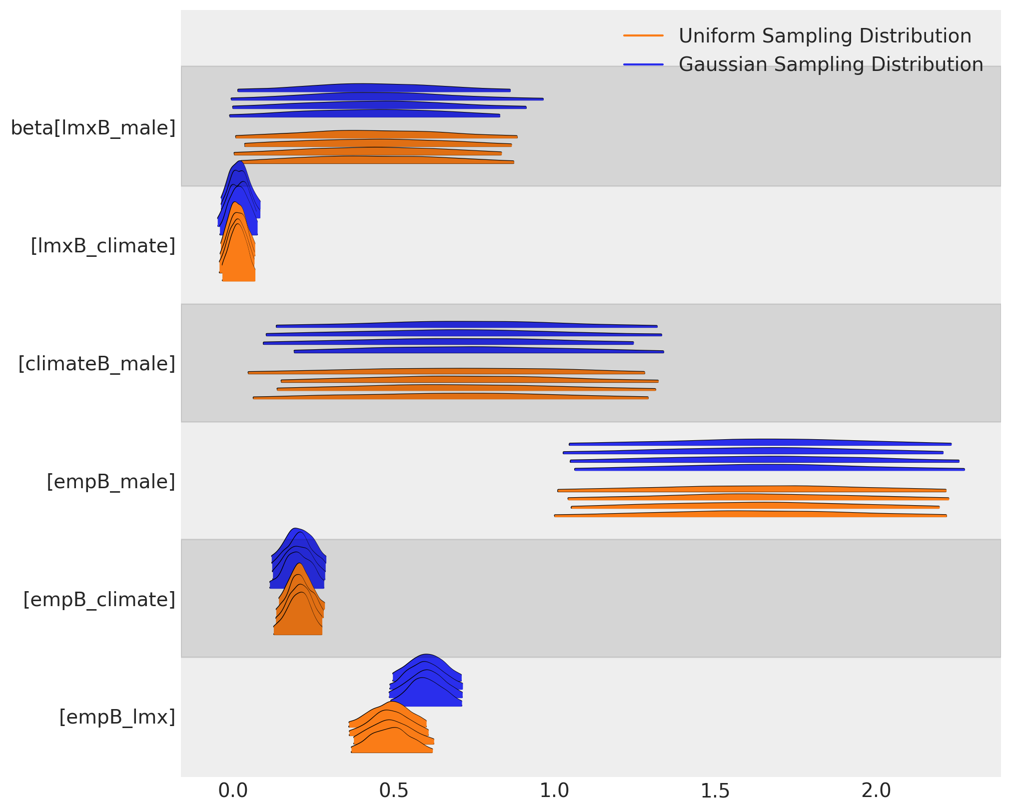
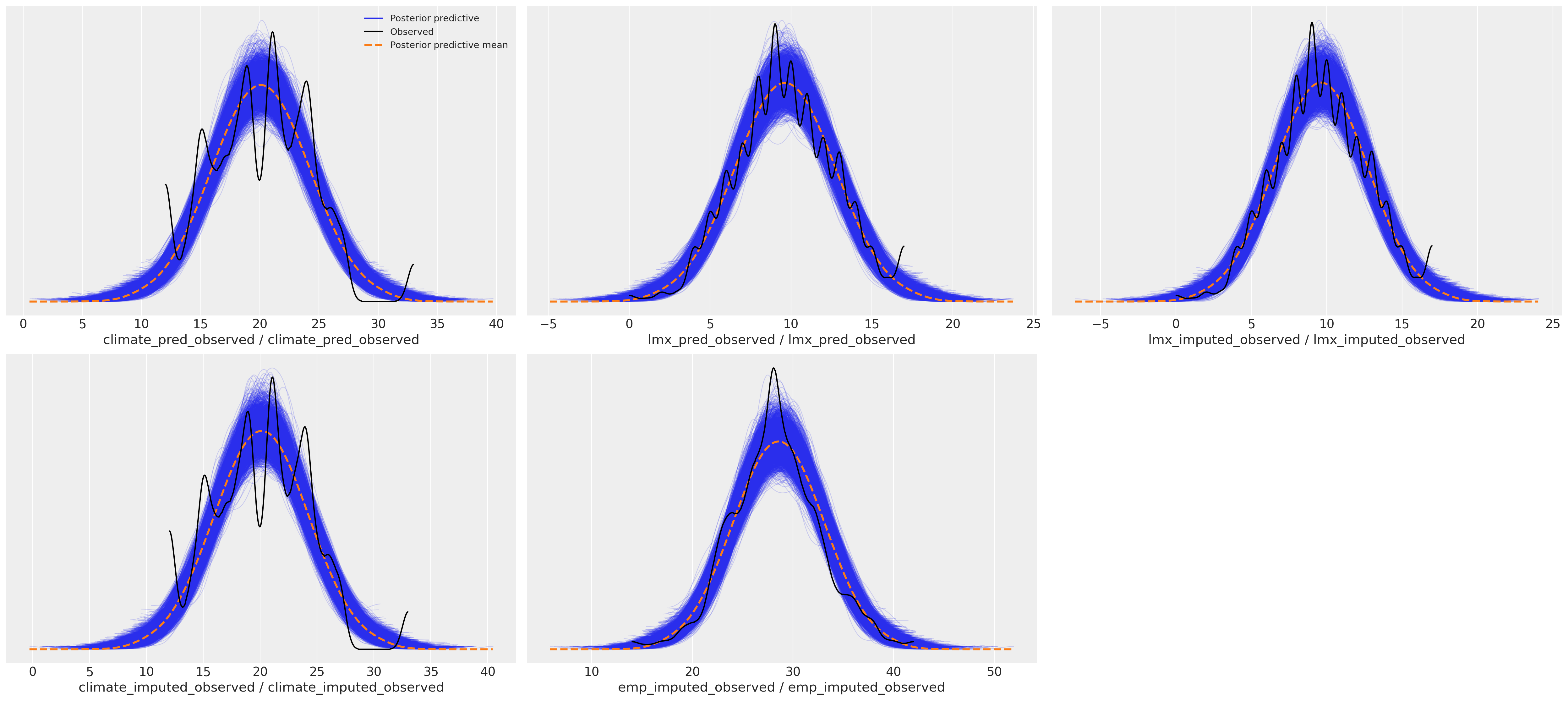
../_images/4adbd352ae483743aee1300261206d8994413c3b4fe7e69bfd18b255d4fcd583.png

This difference has downstream effects on the posterior predictive distribution. We can see here how the sampling distribution for the predictor terms influences the posterior predictive fits on our focal regression equation.

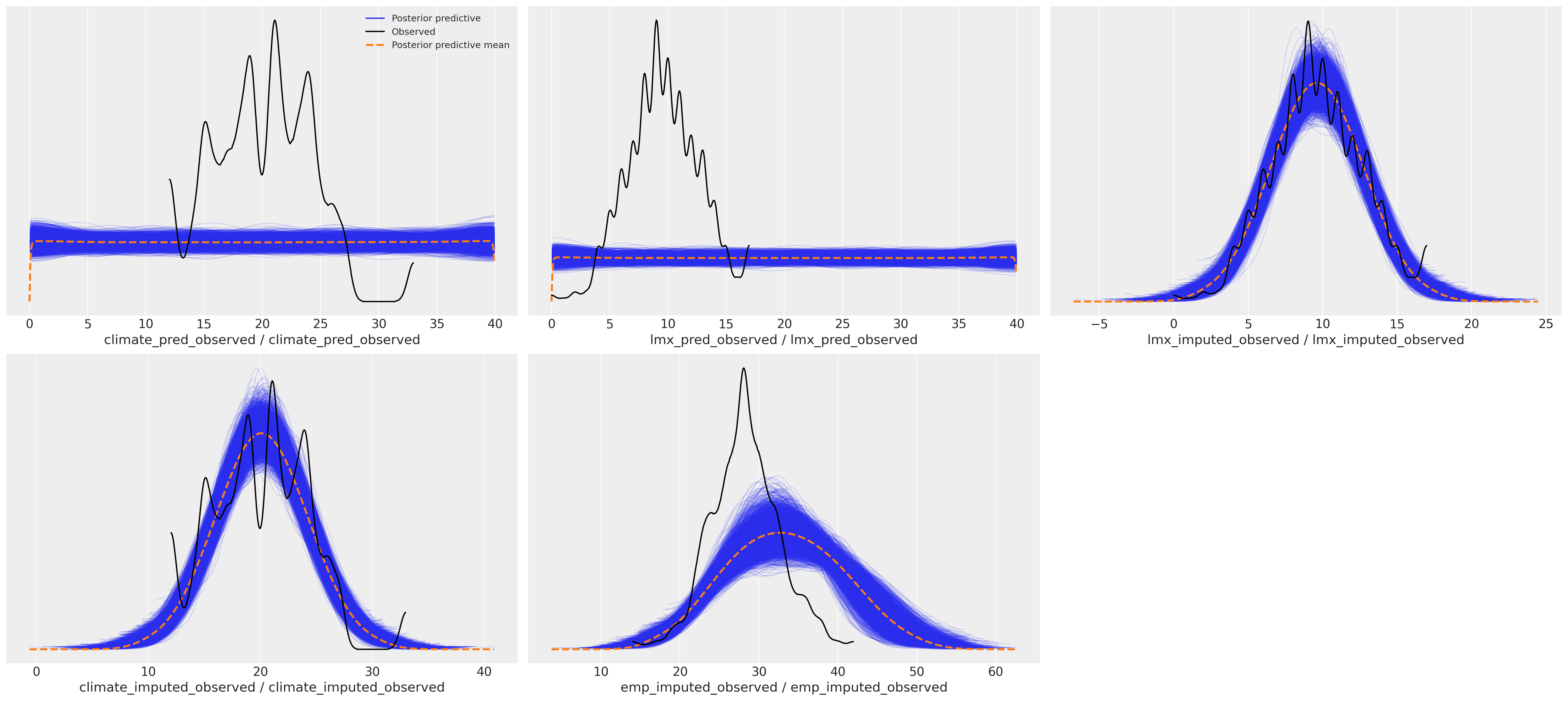
Posterior Predictive Distributions#

az.plot_ppc(idata_uniform)

array([[<AxesSubplot: xlabel='climate_pred_observed / climate_pred_observed'>,
        <AxesSubplot: xlabel='lmx_pred_observed / lmx_pred_observed'>,
        <AxesSubplot: xlabel='lmx_imputed_observed / lmx_imputed_observed'>],
       [<AxesSubplot: xlabel='climate_imputed_observed / climate_imputed_observed'>,
        <AxesSubplot: xlabel='emp_imputed_observed / emp_imputed_observed'>,
        <AxesSubplot: >]], dtype=object)

../_images/041a30ea88dfd5bff20af9e8ea944068fe90f11148fbad487df15bd04daaf7a2.png

az.plot_ppc(idata_normal)

array([[<AxesSubplot: xlabel='climate_pred_observed / climate_pred_observed'>,
        <AxesSubplot: xlabel='lmx_pred_observed / lmx_pred_observed'>,
        <AxesSubplot: xlabel='lmx_imputed_observed / lmx_imputed_observed'>],
       [<AxesSubplot: xlabel='climate_imputed_observed / climate_imputed_observed'>,
        <AxesSubplot: xlabel='emp_imputed_observed / emp_imputed_observed'>,
        <AxesSubplot: >]], dtype=object)

../_images/433326c3305d7a1842db998532dcf019425654f22a3615776cdfe87de50773c0.png

Process the Posterior Predictive Distribution#

Above we estimated a number of likelihood terms in a single PyMC model context. These likelihoods constrained the hyper-parameters which determined the imputation values of the missing terms in the variables used as predictors in our focal regression equation for empower. But we could also perform a more manual sequential imputation, where we model each of the subordinate regression equations seperately and extract the imputed values for each variable in turn and then run a simple regression on the imputed values for the focal regression equation.

We show here how to extract the imputed values for each of the regression equations and augment the observed data.

def get_imputed(idata, data):
    imputed_data = data.copy()
    imputed_climate = az.extract(idata, group="posterior_predictive", num_samples=1000)[
        "climate_imputed"
    ].mean(axis=1)
    mask = imputed_data["climate"].isnull()
    imputed_data.loc[mask, "climate"] = imputed_climate.values[imputed_data[mask].index]

    imputed_lmx = az.extract(idata, group="posterior_predictive", num_samples=1000)[
        "lmx_imputed"
    ].mean(axis=1)
    mask = imputed_data["lmx"].isnull()
    imputed_data.loc[mask, "lmx"] = imputed_lmx.values[imputed_data[mask].index]

    imputed_emp = az.extract(idata, group="posterior_predictive", num_samples=1000)[
        "emp_imputed"
    ].mean(axis=1)
    mask = imputed_data["empower"].isnull()
    imputed_data.loc[mask, "empower"] = imputed_emp.values[imputed_data[mask].index]
    assert imputed_data.isnull().sum().to_list() == [0, 0, 0, 0]
    imputed_data.columns = ["imputed_" + col for col in imputed_data.columns]
    return imputed_data


imputed_data_uniform = get_imputed(idata_uniform, data)
imputed_data_normal = get_imputed(idata_normal, data)
imputed_data_normal.head(5)

	imputed_lmx	imputed_empower	imputed_climate	imputed_male
0	11.0	32.000000	18.0	1
1	13.0	29.490539	18.0	1
2	9.0	30.000000	18.0	1
3	8.0	29.000000	18.0	1
4	7.0	26.000000	18.0	0

We used the mean here to impute the expected value for each missing cell, but you could perform a kind of sensitivity analysis using the many plausible values in posterior predictive distribution

Plotting the Imputed Datasets#

Now we’ll plot the imputed values against their observed values to show how the different sampling distributions impact the pattern of imputation.

joined_uniform = pd.concat([imputed_data_uniform, data], axis=1)
joined_normal = pd.concat([imputed_data_normal, data], axis=1)
for col in ["lmx", "empower", "climate"]:
    joined_uniform[col + "_missing"] = np.where(joined_uniform[col].isnull(), 1, 0)
    joined_normal[col + "_missing"] = np.where(joined_normal[col].isnull(), 1, 0)


def rand_jitter(arr):
    stdev = 0.01 * (max(arr) - min(arr))
    return arr + np.random.randn(len(arr)) * stdev


fig, axs = plt.subplots(1, 3, figsize=(20, 8))
axs = axs.flatten()
ax = axs[0]
ax1 = axs[1]
ax2 = axs[2]

## Derived from MV norm fit.
z = multivariate_normal(
    [lmx_mean, joined_uniform["imputed_empower"].mean()], [[8.9, 5.4], [5.4, 19]]
).pdf(joined_uniform[["imputed_lmx", "imputed_empower"]])

ax.scatter(
    rand_jitter(joined_uniform["imputed_lmx"]),
    rand_jitter(joined_uniform["imputed_empower"]),
    c=joined_uniform["empower_missing"],
    cmap=cm.winter,
    ec="black",
    s=50,
)
ax.set_title("Relationship between LMX and Empowerment \n after Uniform Imputation", fontsize=20)
ax.tricontour(joined_uniform["imputed_lmx"], joined_uniform["imputed_empower"], z)
ax.set_xlabel("Leader-Member-Exchange")
ax.set_ylabel("Empowerment")


custom_lines = [
    Line2D([0], [0], color=cm.winter(0.0), lw=4),
    Line2D([0], [0], color=cm.winter(0.9), lw=4),
]
ax.legend(custom_lines, ["Observed", "Missing - Imputed Empowerment Values"])

z = multivariate_normal(
    [lmx_mean, joined_normal["imputed_empower"].mean()], [[8.9, 5.4], [5.4, 19]]
).pdf(joined_normal[["imputed_lmx", "imputed_empower"]])

ax2.scatter(
    rand_jitter(joined_normal["imputed_lmx"]),
    rand_jitter(joined_normal["imputed_empower"]),
    c=joined_normal["empower_missing"],
    cmap=cm.autumn,
    ec="black",
    s=50,
)
ax2.set_title("Relationship between LMX and Empowerment \n after Gaussian Imputation", fontsize=20)
ax2.tricontour(joined_normal["imputed_lmx"], joined_normal["imputed_empower"], z)
ax2.set_xlabel("Leader-Member-Exchange")
ax2.set_ylabel("Empowerment")
custom_lines = [
    Line2D([0], [0], color=cm.autumn(0.0), lw=4),
    Line2D([0], [0], color=cm.autumn(0.9), lw=4),
]
ax2.legend(custom_lines, ["Observed", "Missing - Imputed Empowerment Values"])

ax1.hist(
    joined_normal["imputed_empower"],
    label="Gaussian Imputed Empowerment",
    bins=30,
    color="slateblue",
    ec="black",
)
ax1.hist(
    joined_uniform["imputed_empower"],
    label="Uniform Imputed Empowerment",
    bins=30,
    color="cyan",
    ec="black",
)
ax1.hist(
    joined_normal["empower"], label="Observed Empowerment", bins=30, color="magenta", ec="black"
)
ax1.legend()
ax1.set_title("Imputed & Observed Empowerment", fontsize=20);

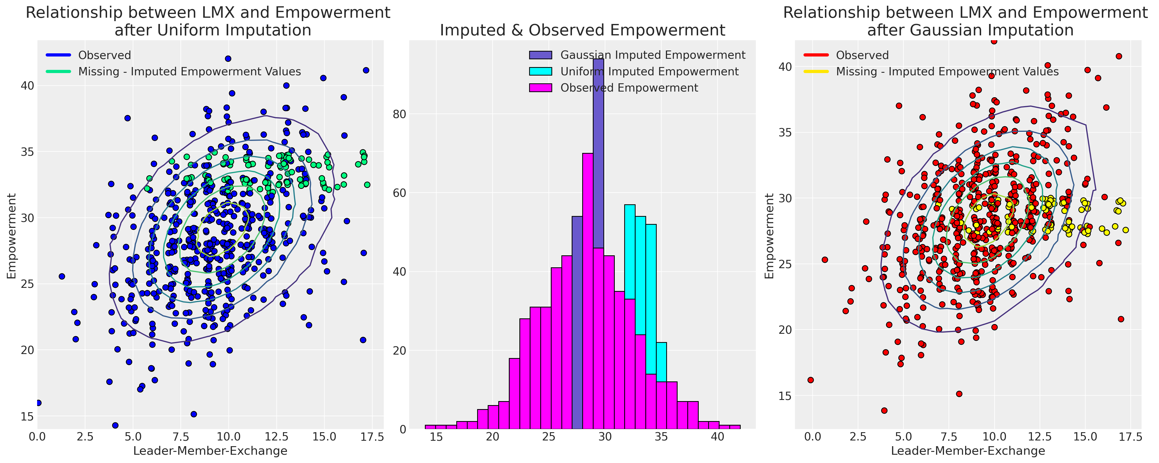
../_images/fd129105d790df8ed2b4ccfb93f673787aeccd985670216a7ee734230ee95a76.png

Ultimately our choice of sampling distribution leads to differently plausible imputations. The choice of which model to go with will driven by the assumptions which govern the reasons for missing-ness in our data.

Hierarchical Structures and Data Imputation#

Our employee dataset has more fine-grained structure than we’ve examined so far. In particular there are 100 or so teams which make up our employee pool, and we might wonder to what degree the propensity for satisfaction or incomplete survey scores are due to the local team environments? Could this be a factor in our patterns of missing data? We’ll examine the reported empowerment scores by team and plot the regression lines by as predicted within each team by their reported lmx score.

heatmap = df_employee.pivot("employee", "team", "empower").dropna(how="all")
heatmap = pd.concat(
    [heatmap[~heatmap[col].isnull()][col].reset_index(drop=True) for col in heatmap.columns], axis=1
)
with pd.option_context("format.precision", 2):
    display(heatmap.style.background_gradient(cmap="Blues"));

/var/folders/99/gp2xl6x513s0tvl3cx79zf7m0000gn/T/ipykernel_96943/1805800404.py:1: FutureWarning: In a future version of pandas all arguments of DataFrame.pivot will be keyword-only.
  heatmap = df_employee.pivot("employee", "team", "empower").dropna(how="all")

	1	2	3	4	5	6	7	8	9	10	11	12	13	14	15	16	17	18	19	20	21	22	23	24	25	26	27	28	29	30	31	32	33	34	35	36	37	38	39	40	41	42	43	44	45	46	47	48	49	50	51	52	53	54	55	56	57	58	59	60	61	62	63	64	65	66	67	68	69	70	71	72	73	74	75	76	77	78	79	80	81	82	83	84	85	86	87	88	89	90	91	92	93	94	95	96	97	98	99	100	101	102	103	104	105
0	32.00	22.00	16.00	26.00	33.00	21.00	29.00	26.00	27.00	33.00	28.00	36.00	24.00	24.00	34.00	28.00	29.00	22.00	28.00	23.00	25.00	39.00	28.00	28.00	26.00	29.00	34.00	25.00	30.00	26.00	28.00	23.00	32.00	27.00	38.00	22.00	36.00	30.00	30.00	30.00	30.00	28.00	27.00	28.00	25.00	21.00	37.00	24.00	31.00	27.00	28.00	32.00	27.00	30.00	28.00	26.00	29.00	20.00	30.00	27.00	32.00	22.00	32.00	31.00	26.00	29.00	24.00	23.00	33.00	29.00	35.00	25.00	33.00	23.00	32.00	27.00	31.00	28.00	27.00	28.00	25.00	31.00	28.00	31.00	28.00	32.00	24.00	29.00	28.00	30.00	33.00	23.00	28.00	21.00	25.00	39.00	25.00	31.00	30.00	24.00	29.00	25.00	20.00	28.00	28.00
1	30.00	23.00	25.00	27.00	37.00	29.00	26.00	25.00	28.00	27.00	26.00	32.00	23.00	30.00	24.00	24.00	26.00	28.00	33.00	22.00	17.00	31.00	22.00	36.00	34.00	23.00	32.00	30.00	30.00	22.00	22.00	28.00	31.00	30.00	32.00	23.00	32.00	36.00	23.00	26.00	24.00	32.00	36.00	26.00	25.00	35.00	32.00	28.00	24.00	28.00	35.00	28.00	32.00	24.00	26.00	23.00	26.00	29.00	28.00	28.00	33.00	29.00	25.00	28.00	27.00	29.00	24.00	34.00	27.00	28.00	31.00	27.00	25.00	30.00	28.00	20.00	28.00	32.00	23.00	15.00	29.00	31.00	31.00	28.00	30.00	28.00	40.00	30.00	26.00	19.00	25.00	23.00	32.00	27.00	30.00	26.00	35.00	24.00	25.00	23.00	28.00	34.00	26.00	28.00	17.00
2	29.00	32.00	31.00	42.00	29.00	25.00	26.00	29.00	26.00	29.00	30.00	30.00	25.00	22.00	21.00	34.00	33.00	32.00	26.00	29.00	35.00	32.00	33.00	27.00	26.00	22.00	29.00	29.00	32.00	30.00	35.00	29.00	33.00	30.00	30.00	31.00	26.00	28.00	40.00	25.00	41.00	27.00	23.00	31.00	29.00	28.00	27.00	23.00	36.00	28.00	23.00	31.00	29.00	33.00	27.00	19.00	25.00	33.00	29.00	27.00	23.00	28.00	31.00	26.00	22.00	37.00	24.00	33.00	37.00	29.00	29.00	26.00	27.00	31.00	23.00	14.00	28.00	30.00	29.00	28.00	36.00	27.00	28.00	35.00	29.00	38.00	26.00	38.00	30.00	34.00	38.00	28.00	34.00	28.00	28.00	30.00	31.00	27.00	29.00	24.00	33.00	30.00	28.00	26.00	28.00
3	26.00	36.00	27.00	24.00	32.00	36.00	26.00	27.00	29.00	36.00	28.00	30.00	27.00	27.00	33.00	34.00	29.00	27.00	33.00	26.00	26.00	33.00	30.00	26.00	28.00	31.00	20.00	30.00	23.00	30.00	28.00	25.00	32.00	31.00	18.00	29.00	26.00	26.00	27.00	nan	28.00	nan	29.00	25.00	22.00	33.00	33.00	30.00	33.00	34.00	nan	37.00	29.00	27.00	28.00	23.00	25.00	32.00	21.00	24.00	30.00	29.00	28.00	27.00	24.00	38.00	24.00	19.00	30.00	35.00	32.00	28.00	38.00	31.00	27.00	23.00	30.00	27.00	27.00	27.00	32.00	27.00	29.00	26.00	24.00	29.00	28.00	31.00	25.00	25.00	30.00	29.00	34.00	32.00	31.00	26.00	nan	34.00	27.00	21.00	24.00	25.00	28.00	23.00	32.00
4	nan	nan	30.00	37.00	24.00	nan	31.00	nan	28.00	24.00	28.00	34.00	24.00	38.00	35.00	nan	nan	nan	nan	29.00	37.00	32.00	nan	24.00	nan	26.00	29.00	26.00	35.00	29.00	nan	29.00	nan	nan	nan	20.00	23.00	31.00	22.00	nan	nan	nan	23.00	nan	19.00	nan	32.00	22.00	31.00	27.00	nan	nan	nan	nan	24.00	nan	27.00	28.00	26.00	25.00	30.00	22.00	30.00	28.00	32.00	29.00	28.00	nan	nan	28.00	30.00	nan	28.00	26.00	25.00	nan	27.00	35.00	24.00	29.00	24.00	nan	33.00	28.00	34.00	31.00	22.00	nan	26.00	18.00	32.00	22.00	nan	31.00	33.00	nan	nan	32.00	28.00	21.00	35.00	36.00	31.00	27.00	nan
5	nan	nan	23.00	nan	31.00	nan	33.00	nan	25.00	22.00	25.00	nan	nan	30.00	23.00	nan	nan	nan	nan	24.00	nan	31.00	nan	nan	nan	nan	nan	nan	nan	32.00	nan	25.00	nan	nan	nan	20.00	31.00	25.00	nan	nan	nan	nan	nan	nan	28.00	nan	nan	27.00	27.00	nan	nan	nan	nan	nan	27.00	nan	31.00	29.00	nan	31.00	nan	30.00	nan	nan	nan	nan	nan	nan	nan	nan	28.00	nan	nan	nan	nan	nan	33.00	30.00	19.00	23.00	nan	nan	26.00	28.00	26.00	nan	nan	nan	28.00	30.00	36.00	24.00	nan	nan	29.00	nan	nan	nan	28.00	27.00	28.00	31.00	24.00	nan	nan

fits = []
x = np.linspace(0, 20, 100)
fig, ax = plt.subplots(figsize=(20, 7))
for team in df_employee["team"].unique():
    temp = df_employee[df_employee["team"] == team][["lmx", "empower"]].dropna()
    fit = np.polyfit(temp["lmx"], temp["empower"], 1)
    y = fit[0] * x + fit[1]
    fits.append(fit)
    ax.plot(x, y, alpha=0.6)
    ax.scatter(rand_jitter(temp["lmx"]), rand_jitter(temp["empower"]), color="black", ec="white")
ax.set_title("Simple Regression fits by Team \n Empower ~ LMX", fontsize=20)
ax.set_xlabel("Leader-Member-Exchange (LMX)")
ax.set_ylabel("Empowerment")
ax.set_ylim(0, 45);

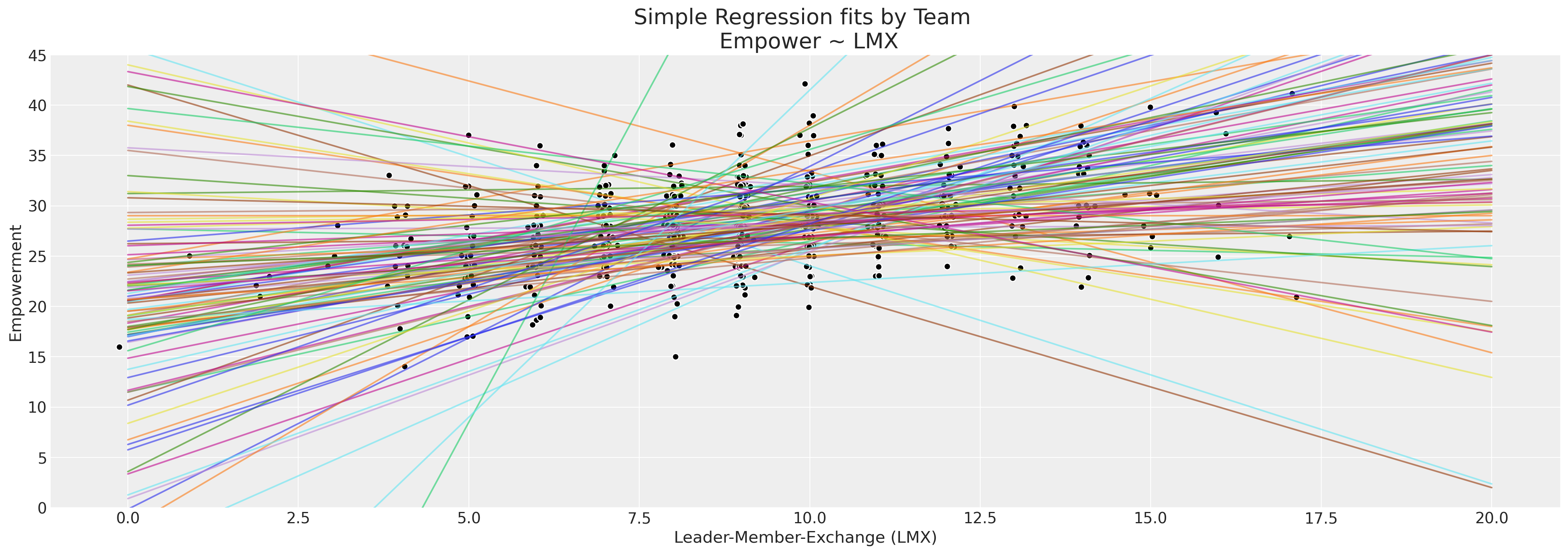
../_images/158b68f573895eb344521f181e0fa3d88f550f3581e4ff54bea36ceabd47fc98.png

There is enough spread in the regression lines to at least suggest that there is a heterogenous relationship between empowerment and the work environment as we look across different teams, but limited observations in each team. This is a perfect use case for a hierarchical bayesian model.

team_idx, teams = pd.factorize(df_employee["team"], sort=True)
employee_idx, _ = pd.factorize(df_employee["employee"], sort=True)
coords = {"team": teams, "employee": np.arange(len(df_employee))}


with pm.Model(coords=coords) as hierarchical_model:
    # Priors
    company_beta_lmx = pm.Normal("company_beta_lmx", 0, 1)
    company_beta_male = pm.Normal("company_beta_male", 0, 1)
    company_alpha = pm.Normal("company_alpha", 20, 2)
    team_alpha = pm.Normal("team_alpha", 0, 1, dims="team")
    team_beta_lmx = pm.Normal("team_beta_lmx", 0, 1, dims="team")
    sigma = pm.HalfNormal("sigma", 4, dims="employee")

    # Imputed Predictors
    mu_lmx = pm.Normal("mu_lmx", 10, 5)
    sigma_lmx = pm.HalfNormal("sigma_lmx", 5)
    lmx_pred = pm.Normal("lmx_pred", mu_lmx, sigma_lmx, observed=df_employee["lmx"].values)

    # Combining Levels
    alpha_global = pm.Deterministic("alpha_global", company_alpha + team_alpha[team_idx])
    beta_global_lmx = pm.Deterministic(
        "beta_global_lmx", company_beta_lmx + team_beta_lmx[team_idx]
    )
    beta_global_male = pm.Deterministic("beta_global_male", company_beta_male)

    # Likelihood
    mu = pm.Deterministic(
        "mu",
        alpha_global + beta_global_lmx * lmx_pred + beta_global_male * df_employee["male"].values,
    )

    empower_imputed = pm.Normal(
        "emp_imputed",
        mu,
        sigma,
        observed=df_employee["empower"].values,
    )

    idata_hierarchical = pm.sample_prior_predictive()
    # idata_hierarchical.extend(pm.sample(random_seed=1200, target_accept=0.99))
    idata_hierarchical.extend(
        sample_blackjax_nuts(draws=20_000, random_seed=500, target_accept=0.99)
    )
    pm.sample_posterior_predictive(idata_hierarchical, extend_inferencedata=True)

pm.model_to_graphviz(hierarchical_model)

/Users/nathanielforde/opt/miniconda3/envs/missing_data_clean/lib/python3.11/site-packages/pymc/model.py:1400: ImputationWarning: Data in lmx_pred contains missing values and will be automatically imputed from the sampling distribution.
  warnings.warn(impute_message, ImputationWarning)
/Users/nathanielforde/opt/miniconda3/envs/missing_data_clean/lib/python3.11/site-packages/pymc/model.py:1400: ImputationWarning: Data in emp_imputed contains missing values and will be automatically imputed from the sampling distribution.
  warnings.warn(impute_message, ImputationWarning)
Sampling: [company_alpha, company_beta_lmx, company_beta_male, emp_imputed_missing, emp_imputed_observed, lmx_pred_missing, lmx_pred_observed, mu_lmx, sigma, sigma_lmx, team_alpha, team_beta_lmx]

Compiling...
Compilation time =  0:00:04.523249
Sampling...
Sampling time =  0:00:12.370856
Transforming variables...
Transformation time =  0:12:51.685820

Sampling: [emp_imputed_missing, emp_imputed_observed, lmx_pred_observed]

100.00% [80000/80000 00:21<00:00]

../_images/a904161ef3d90eb781a125bc7ad859272f225587ab9aeb6d113c7a8ef9cb5556.svg

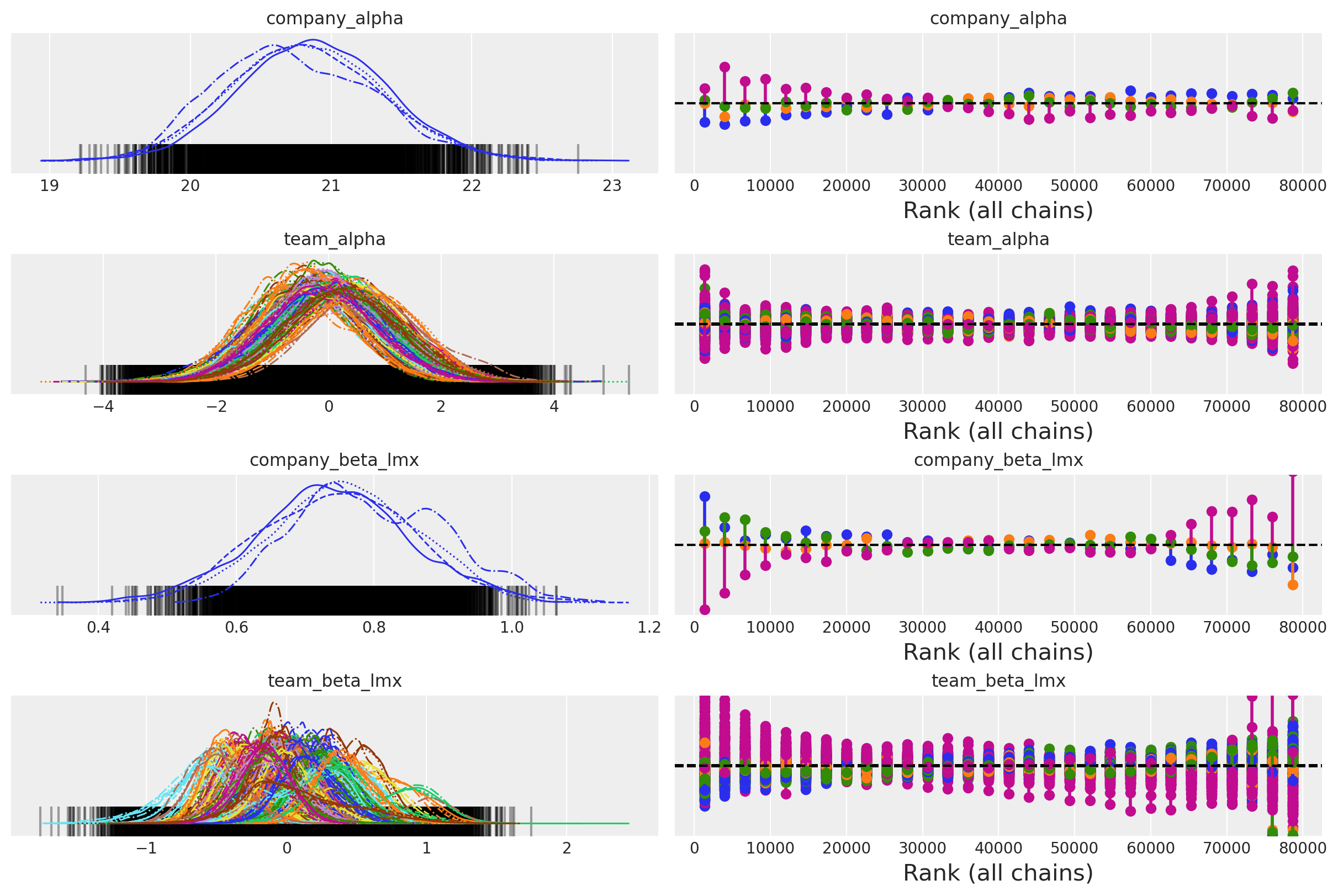
Some Convergence Checks#

az.plot_trace(
    idata_hierarchical,
    var_names=["company_alpha", "team_alpha", "company_beta_lmx", "team_beta_lmx"],
    kind="rank_vlines",
);

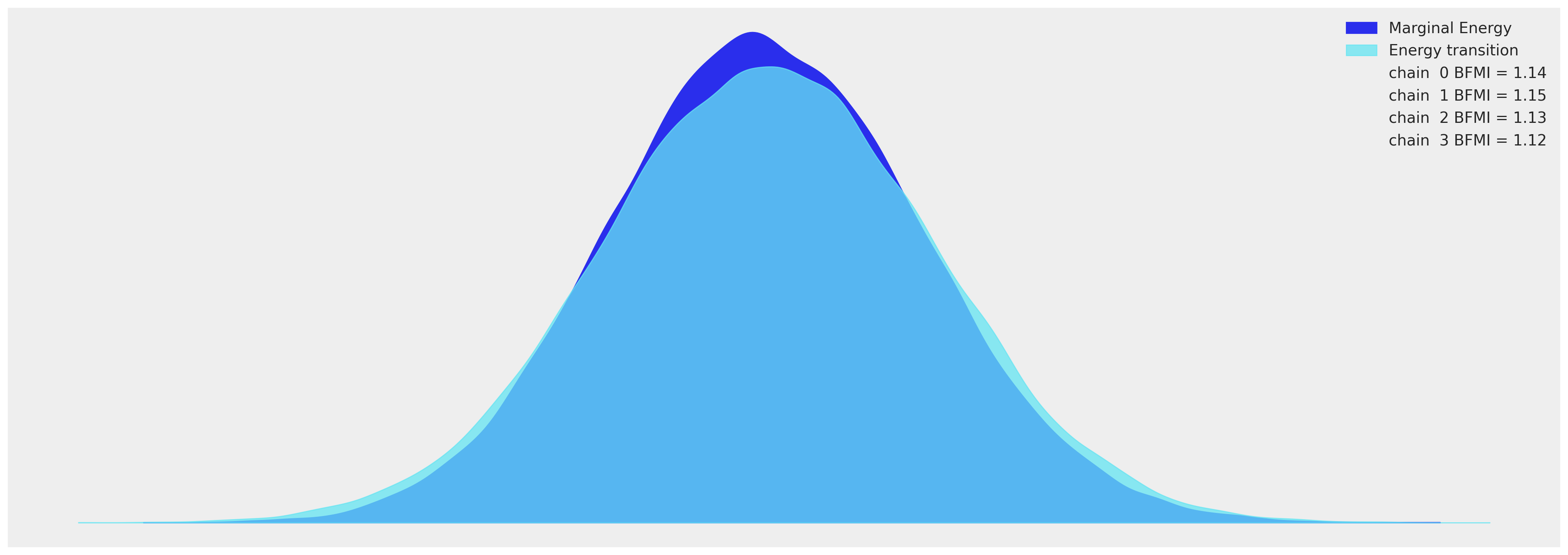
../_images/c795ab0ed51543fe98bc704a3e7fa62556d767cc54a34d1118293b27af4f9a78.png

az.plot_energy(idata_hierarchical, figsize=(20, 7));

../_images/01c8df84ffb5fc5c77276a2af4d0444327e38cf5a06908b4a02c3678bde2e6a4.png

Inspecting the Model Fit#

summary = az.summary(
    idata_hierarchical,
    var_names=[
        "company_alpha",
        "team_alpha",
        "company_beta_lmx",
        "company_beta_male",
        "team_beta_lmx",
    ],
)

summary

	mean	sd	hdi_3%	hdi_97%	mcse_mean	mcse_sd	ess_bulk	ess_tail	r_hat
company_alpha	20.818	0.545	19.806	21.840	0.029	0.020	358.0	1316.0	1.02
team_alpha[1]	-0.214	0.955	-1.975	1.604	0.030	0.021	1043.0	2031.0	1.00
team_alpha[2]	-0.067	0.995	-1.975	1.772	0.026	0.018	1496.0	2572.0	1.00
team_alpha[3]	-0.568	0.931	-2.271	1.250	0.027	0.019	1144.0	2135.0	1.00
team_alpha[4]	-0.228	0.993	-2.085	1.630	0.025	0.018	1552.0	4305.0	1.00
...	...	...	...	...	...	...	...	...	...
team_beta_lmx[101]	0.157	0.207	-0.226	0.550	0.010	0.007	436.0	872.0	1.01
team_beta_lmx[102]	0.407	0.198	0.042	0.785	0.011	0.008	338.0	876.0	1.01
team_beta_lmx[103]	-0.146	0.213	-0.549	0.253	0.014	0.010	215.0	835.0	1.03
team_beta_lmx[104]	-0.167	0.187	-0.517	0.186	0.010	0.007	338.0	1346.0	1.01
team_beta_lmx[105]	0.071	0.393	-0.562	0.902	0.021	0.015	390.0	476.0	1.01

213 rows × 9 columns

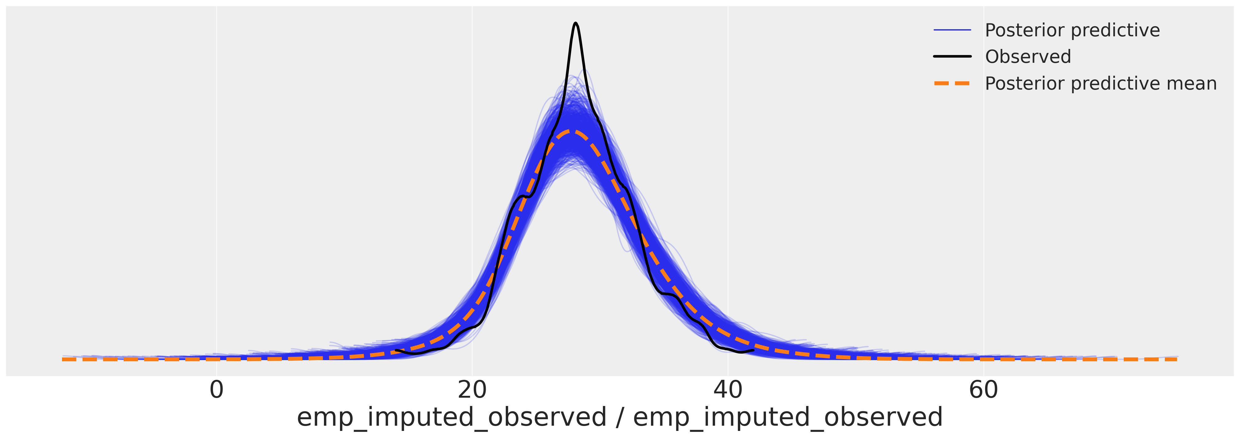
az.plot_ppc(
    idata_hierarchical, var_names=["emp_imputed_observed"], figsize=(20, 7), num_pp_samples=1000
)

<AxesSubplot: xlabel='emp_imputed_observed / emp_imputed_observed'>

../_images/fcf5a8a9bb124afc3fd9d56a085ecf853c5063f8bd0d86f39f38b3646e2945d3.png

Heterogenous Patterns of Imputation#

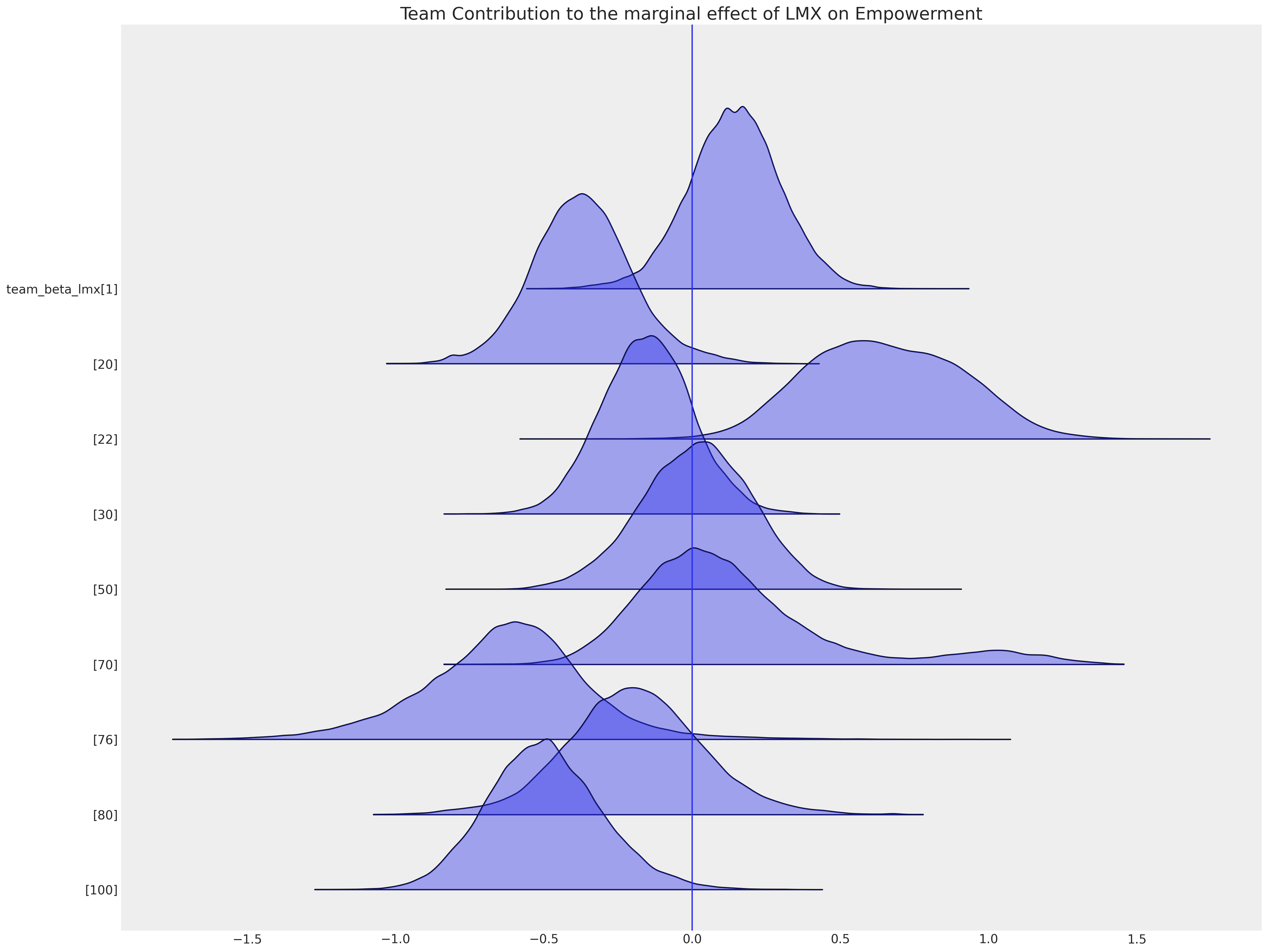
Just as when we consider questions of causal inference and we attend to the confounding influence of local factors, this is also required when we do imputation. We show here a selection of team specific intercept terms which suggest that belonging to a particular team can shift your empowerment above or below the grand mean of the company level intercept term. These local effects of environment are what we seek to account for when imputing missing values.

ax = az.plot_forest(
    idata_hierarchical,
    var_names=["team_beta_lmx"],
    coords={"team": [1, 20, 22, 30, 50, 70, 76, 80, 100]},
    figsize=(20, 15),
    kind="ridgeplot",
    combined=True,
    ridgeplot_alpha=0.4,
    hdi_prob=True,
)
ax[0].axvline(0)
ax[0].set_title("Team Contribution to the marginal effect of LMX on Empowerment", fontsize=20);

../_images/fac7e4d367781ca36e4d4cd9bb78116fea15748d3f8fd44e5980e11e40d38d85.png

The ability to capture this local variation impacts the pattern of imputed values too.

imputed_data = df_employee[["lmx", "empower", "climate"]]

imputed_lmx = az.extract(idata_hierarchical, group="posterior_predictive", num_samples=1000)[
    "lmx_pred"
].mean(axis=1)
mask = imputed_data["lmx"].isnull()
imputed_data.loc[mask, "lmx"] = imputed_lmx.values[imputed_data[mask].index]

imputed_emp = az.extract(idata_hierarchical, group="posterior_predictive", num_samples=1000)[
    "emp_imputed"
].mean(axis=1)
mask = imputed_data["empower"].isnull()
imputed_data.loc[mask, "empower"] = imputed_emp.values[imputed_data[mask].index]
imputed_data.columns = ["imputed_" + col for col in imputed_data.columns]
joined = pd.concat([imputed_data, df_employee], axis=1)
joined["check"] = np.where(joined["empower"].isnull(), 1, 0)

mosaic = """AAAABB"""
fig, axs = plt.subplot_mosaic(mosaic, sharex=False, figsize=(20, 7))
axs = [axs[k] for k in axs.keys()]
axs[0].scatter(
    joined["imputed_lmx"],
    joined["imputed_empower"],
    c=joined["check"],
    cmap=cm.winter,
    ec="black",
    s=40,
)

z = multivariate_normal([10, joined["imputed_empower"].mean()], [[8.9, 5.4], [5.4, 19]]).pdf(
    joined[["imputed_lmx", "imputed_empower"]]
)
axs[0].tricontour(joined["imputed_lmx"], joined["imputed_empower"], z)

axs[1].hist(joined["imputed_empower"], ec="black", label="Imputed", color="limegreen", bins=30)
axs[1].hist(joined["empower"], ec="black", label="observed", color="blue", bins=30)
axs[1].set_title("Empowerment Distributions Imputed  \n with Team Informed Estimates", fontsize=20)
axs[0].set_xlabel("Leader Member Exchange - LMX")
axs[0].set_ylabel("Empowerment")
axs[0].set_title("Empowerment Imputed \n with Team Informed Estimates", fontsize=20)
axs[1].legend();

/var/folders/99/gp2xl6x513s0tvl3cx79zf7m0000gn/T/ipykernel_96943/3267370214.py:7: SettingWithCopyWarning: 
A value is trying to be set on a copy of a slice from a DataFrame

See the caveats in the documentation: https://pandas.pydata.org/pandas-docs/stable/user_guide/indexing.html#returning-a-view-versus-a-copy
  imputed_data.loc[mask, "lmx"] = imputed_lmx.values[imputed_data[mask].index]
/var/folders/99/gp2xl6x513s0tvl3cx79zf7m0000gn/T/ipykernel_96943/3267370214.py:13: SettingWithCopyWarning: 
A value is trying to be set on a copy of a slice from a DataFrame

See the caveats in the documentation: https://pandas.pydata.org/pandas-docs/stable/user_guide/indexing.html#returning-a-view-versus-a-copy
  imputed_data.loc[mask, "empower"] = imputed_emp.values[imputed_data[mask].index]

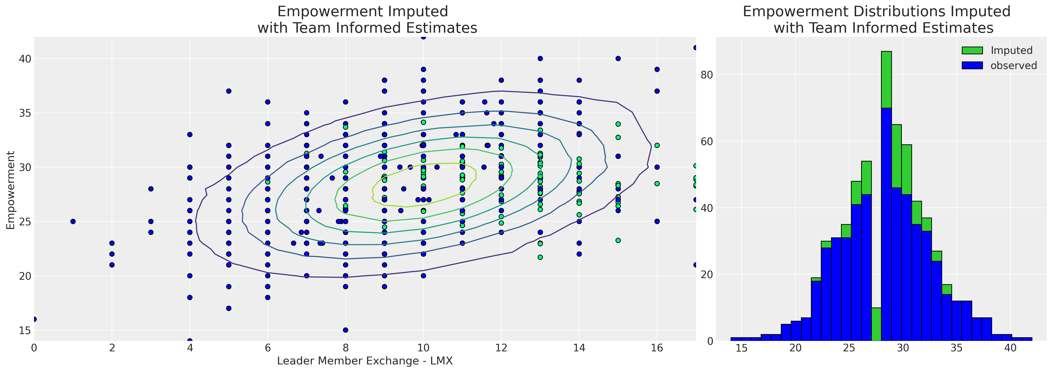
../_images/ae2a5c76f4fe9804a644bf7c043e71fa68a41e69ee1690b518f901dd3f6e1612.png

It’s clear from the hierarchical model that the team specific information has allowed us to impute a wider range of empowerment values with a broader spread as a function of lmx and male. This is much more persuasive since all politics is local, and this latter model is informed by the conditions of work for each employee. As such, our hierarchical model is able to ascribe a more nuanced view of the probable empowerment values for the missing reports. The hierarchical imputation model “borrows information” in two ways (i) the individual team estimates are pulled toward the global estimates and (ii) the missing values are imputed with respect to our measures of the team dynamics.

Conclusion#

We’ve now seen multiple approaches to the imputation of missing data. We have focused on an example where the reason for the missing data is not immediately obvious given how different employees might very well have different reasons for under-specifying their relationship with management. However the techniques applied here are quite general.

The multivariate normal approaches to imputation works surprisingly well in many cases, but the more cutting edge approach is the sequential specification of chained equations. The Bayesian approach here is state of the art because we are quite free to use more than simple regression models as the component models for our imputation equations. For each equation we can be liberal in our choice of likelihood terms and the priors we allow over the sampling distributions. We can also add hierarchical structure to respect natural clusters in our data in so far as they constrain the patterns of missing data.

This general point is important - the flexibility of the Bayesian approach can be tailored to the appropriate complexity of our theory about why our data is missing. Similar considerations apply to the estimation procedures involved in counterfactual inference. The more developed our theory for why the data is missing (why the world is as it is, and not another way), the more we need a flexible modelling framework to capture the subtleties of the theory. Bayesian modelling is a superb tool for this loop of theory construction and evaluation.

Authors#

Authored by Nathaniel Forde in February 2023 for pymc-examples #500

References#

[1]

Craig Enders K. Applied Missing Data Analysis. The Guilford Press, 2022.

Watermark#

%load_ext watermark
%watermark -n -u -v -iv -w -p pytensor

Last updated: Thu Feb 02 2023

Python implementation: CPython
Python version       : 3.11.0
IPython version      : 8.8.0

pytensor: 2.8.11

sys       : 3.11.0 | packaged by conda-forge | (main, Jan 15 2023, 05:44:48) [Clang 14.0.6 ]
pytensor  : 2.8.11
scipy     : 1.10.0
pymc      : 5.0.1
numpy     : 1.24.1
matplotlib: 3.6.3
arviz     : 0.14.0
pandas    : 1.5.2

Watermark: 2.3.1

Categories

Tags