Bayesian Non-parametric Causal Inference

import arviz as az
import matplotlib.lines as mlines
import matplotlib.patches as mpatches
import matplotlib.pyplot as plt
import networkx as nx
import numpy as np
import pandas as pd
import pymc as pm
import pymc_bart as pmb
import pytensor.tensor as pt
import statsmodels.api as sm
import xarray as xr

from sklearn.ensemble import GradientBoostingRegressor, RandomForestRegressor

%config InlineBackend.figure_format = 'retina'  # high resolution figures
az.style.use("arviz-darkgrid")
rng = np.random.default_rng(42)

Causal Inference and Propensity Scores

There are few claims stronger than the assertion of a causal relationship and few claims more contestable. A naive world model - rich with tenuous connections and non-sequiter implications is characteristic of conspiracy theory and idiocy. On the other hand, a refined and detailed knowledge of cause and effect characterised by clear expectations, plausible connections and compelling counterfactuals, will steer you well through the buzzing, blooming confusion of the world.

Causal inference in an experimental setting awkwardly differs from causal inference in an observational setting. In an experimental setting treatments are assigned randomly. With observational data we never know the mechanism that assigned each subject of the analysis to their treatment. This risks a source of bias due to selection effects confounding the analysis of treatments. A propensity score is the estimated probability of receiving a treatment status (e.g. smoker/non-smoker, divorced/married) for each individual in the population under study. We will recount below how understanding an individual’s propensity-for-treatment can help mitigate that selection bias.

Non-parametric methods for estimating propensity scores and treatment effects are an attempt to remain agnostic about the precise functional relationships and avoid model mispecification. This push stems from the idea that excessive modelling assumptions cultivate an unlovely breeding ground for counfounding errors and should be avoided. See Foundations of Agnostic Statistics Aronow and Miller [2019]. We will ultimately argue that such minimalist “desert landscape” aesthetics shatter against causal questions with real import, where substantive assumptions are needed, even when we can avail of nonparametric approaches.

In this notebook we will explain and motivate the usage of propensity scores in the analysis of causal inference questions. Our focus will be on the manner in which we (a) estimate propensity scores and (b) use them in the analysis of causal questions. We will see how they help avoid risks of selection bias in causal inference and where they can go wrong. This method should be comfortable for the Bayesian analyst who is familiar with weighting and re-weighting their claims with information in the form of priors. Propensity score weighting is just another opportunity to enrich your model with knowledge about the world. We will show how they can be applied directly, and then indirectly in the context of debiasing machine learning approaches to causal inference.

We will illustrate these patterns using two data sets: the NHEFS data used in Causal Inference: What If Hernán and Robins [2020], and a second patient focused data set analysed in Bayesian Nonparametrics for Causal Inference and Missing Data Daniels et al. [2024]. The contrast between non-parametric BART models with simpler regression models for the estimation of propensity scores and causal effects will be emphasised.

Note on Propensity Score Matching

Propensity scores are often synonymous with the technique of propensity score matching. We will not be covering this topic. It is a natural extension of propensity score modelling but to our mind introduces complexity through the requirements around (a) choosing a matching algorithm and (b) the information loss with reduced sample size.

The Structure of the Presentation

Below we’ll see a number of examples of non-parametric approaches to the estimation of causal effects. Some of these methods will work well, and others will mislead us. We will demonstrate how these methods serve as tools for imposing stricter and stricter assumptions on our inferential framework. Throughout we will use the potential outcomes notation to discuss causal inference - we draw extensively on work in Aronow and Miller [2019], which can be consulted for more details. But very briefly, when we want to discuss the causal impact of a treatment status on an outcome \(Y\) we will denote the outcome \(Y(t)\) as the outcome measure \(Y\) under the treatment regime \(T = t\).

• Application of Propensity Scores to Selection Effect Bias

  • NHEFS data on weight loss and the relationship to smoking

• Application of Propensity Scores to Selection Effect Bias

  • Health Expenditure Data and the relationship to smoking

• Application of Debiased/Double ML to estimate ATE

• Application of Mediation Analysis to estimate Direct and Indirect Effects

These escalating set of assumptions required to warrant causal inference under different threats of confounding shed light on the process of inference as a whole.

Why do we care about Propensity Scores?

With observational data we cannot re-run the assignment mechanism but we can estimate it, and transform our data to proportionally weight the data summaries within each group so that the analysis is less effected by the over-representation of different strata in each group. This is what we hope to use the propensity scores to achieve.

Firstly, and somewhat superficially, the propensity score is a dimension reduction technique. We take a complex covariate profile \(X_{i}\) representing an individual’s measured attributes and reduce it to a scalar \(p^{i}_{T}(X)\). It is also a tool for thinking about the potential outcomes of an individual under different treatment regimes. In a policy evaluation context it can help partial out the degree of incentives for policy adoption across strata of the population. What drives adoption or assignment in each niche of the population? How can different demographic strata be induced towards or away from adoption of the policy? Understanding these dynamics is crucial to gauge why selection bias might emerge in any sample data. Paul Goldsmith-Pinkham’s lectures are particularly clear on this last point, and why this perspective is appealing to structural econometricians.

The pivotal idea when thinking about propensity scores is that we cannot license causal claims unless (i) the treatment assignment is independent of the covariate profiles i.e \(T \perp\!\!\!\perp X\) and (ii) the outcomes \(Y(0)\), and \(Y(1)\) are similarly conditionally independent of the treatement \(T | X\). If these conditions hold, then we say that \(T\) is strongly ignorable given \(X\). This is also occasionally noted as the unconfoundedness or exchangeability assumption. For each strata of the population defined by the covariate profile \(X\), we require that, after controlling for \(X\), it’s as good as random which treatment status an individual adopts. This means that after controlling for \(X\), any differences in outcomes between the treated and untreated groups can be attributed to the treatment itself rather than confounding variables.

It is a theorem that if \(T\) is strongly ignorable given \(X\), then (i) and (ii) hold given \(p_{T}(X)\) too. So valid statistical inference proceeds in a lower dimensional space using the propensity score as a proxy for the higher dimensional data. This is useful because some of the strata of a complex covariate profile may be sparsely populated so substituting a propensity score enables us to avoid the risks of high dimensional missing data. Causal inference is unconfounded when we have controlled for enough of drivers for policy adoption, that selection effects within each covariate profiles \(X\) seem essentially random. The insight this suggests is that when you want to estimate a causal effect you are only required to control for the covariates which impact the probability of treatement assignment. More concretely, if it’s easier to model the assignment mechanism than the outcome mechanism this can be substituted in the case of causal inference with observed data.

Given the assumption that we are measuring the right covariate profiles to induce strong ignorability, then propensity scores can be used thoughtfully to underwrite causal claims.

Propensity Scores in a Picture

Some methodologists advocate for the analysis of causal claims through the postulation and assessment of directed acyclic graphs which are purported to represent the relationships of causal influence. In the case of propensity score analysis, we have the following picture. Note how the influence of X on the outcome doesn’t change, but its influence on the treatment is bundled into the propensity score metric. Our assumption of strong ignorability is doing all the work to gives us license to causal claims. The propensity score methods enable these moves through the corrective use of the structure bundled into the propensity score.

Show code cell source Hide code cell source

fig, axs = plt.subplots(1, 2, figsize=(20, 15))
axs = axs.flatten()
graph = nx.DiGraph()
graph.add_node("X")
graph.add_node("p(X)")
graph.add_node("T")
graph.add_node("Y")
graph.add_edges_from([("X", "p(X)"), ("p(X)", "T"), ("T", "Y"), ("X", "Y")])
graph1 = nx.DiGraph()
graph1.add_node("X")
graph1.add_node("T")
graph1.add_node("Y")
graph1.add_edges_from([("X", "T"), ("T", "Y"), ("X", "Y")])
nx.draw(
    graph,
    arrows=True,
    with_labels=True,
    pos={"X": (1, 2), "p(X)": (1, 3), "T": (1, 4), "Y": (2, 1)},
    ax=axs[1],
    node_size=6000,
    font_color="whitesmoke",
    font_size=20,
)
nx.draw(
    graph1,
    arrows=True,
    with_labels=True,
    pos={"X": (1, 2), "T": (1, 4), "Y": (2, 1)},
    ax=axs[0],
    node_size=6000,
    font_color="whitesmoke",
    font_size=20,
)

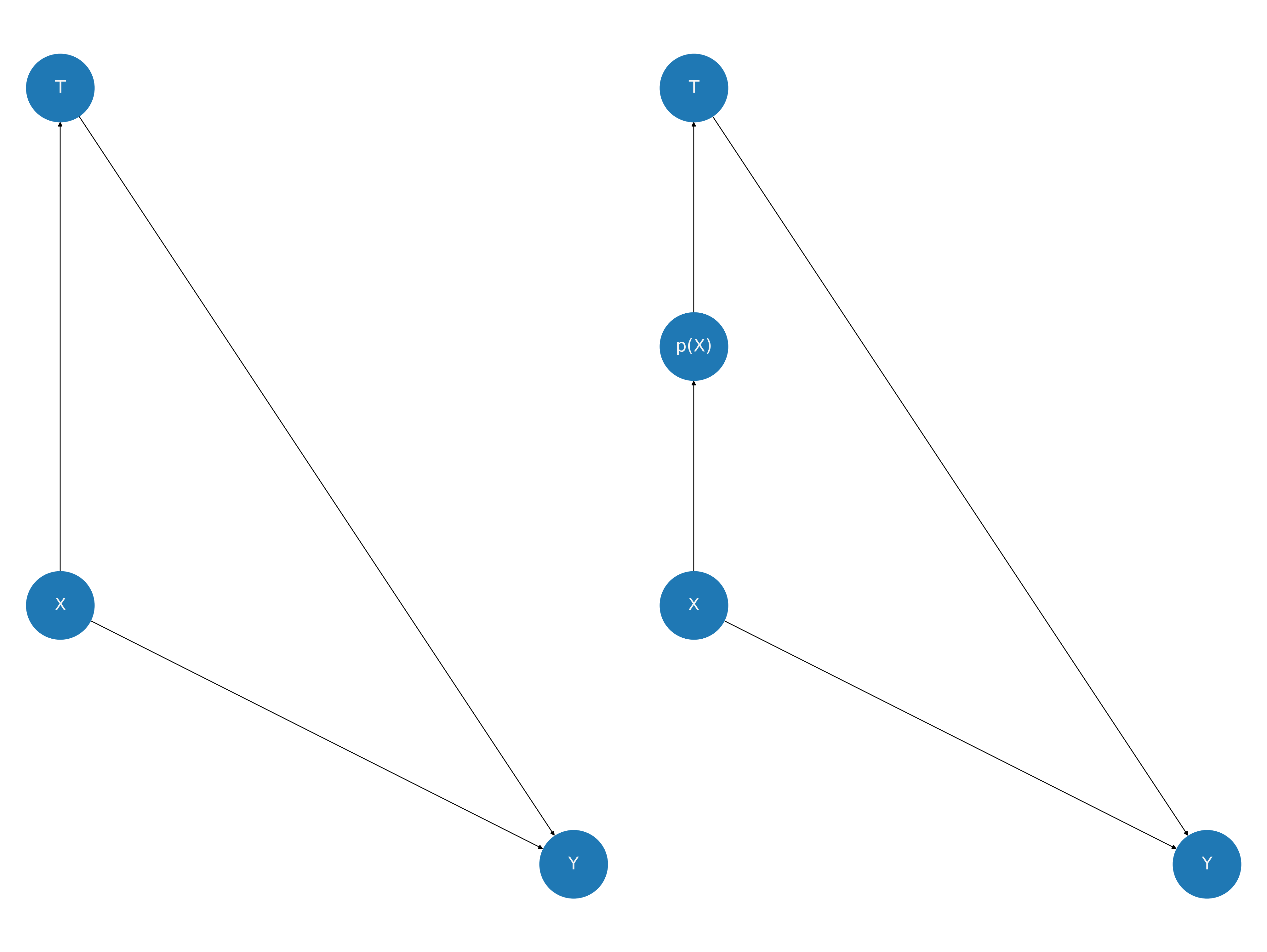
In the above picture we see how the inclusion of a propensity score variable blocks the path between the covariate profile X and the treatment variable T. This is a useful perspective on the assumption of strong ignorability because it implies that \(T \perp\!\!\!\perp X |p(X)\) which implies that the covariate profiles are balanced across the treatment branches conditional on the propensity score. This is a testable implication of the postulated design!

If our treatment status is such that individuals will more or less actively select themselves into the status, then a naive comparisons of differences between treatment groups and control groups will be misleading to the degree that we have over-represented types of individual (covariate profiles) in the population.Randomisation solves this by balancing the covariate profiles across treatment and control groups and ensuring the outcomes are independent of the treatment assignment. But we can’t always randomise. Propensity scores are useful because they can help emulate as-if random assignment of treatment status in the sample data through a specific transformation of the observed data.

This type of assumption and ensuing tests of balance based on propensity scores is often substituted for elaboration of the structural DAG that systematically determine the treatment assignment. The idea being that if we can achieve balance across covariates conditional on a propensity score we have emulated an as-if random allocation we can avoid the hassle of specifying too much structure and remain agnostic about the strucuture of the mechanism. This can often be a useful strategy but, as we will see, elides the specificity of the causal question and the data generating process.

Non-Confounded Inference: NHEFS Data

This data set from the National Health and Nutrition Examination survey records details of weight, activity and smoking habits of around 1500 individuals over two periods. The first period established a baseline and a follow-up period 10 years later. We will analyse whether the individual (trt == 1) quit smoking before the follow up visit. Each individuals’ outcome represents a relative weight gain/loss comparing the two periods.

try:
    nhefs_df = pd.read_csv("../data/nhefs.csv")
except:
    nhefs_df = pd.read_csv(pm.get_data("nhefs.csv"))

nhefs_df.head()

	age	race	sex	smokeintensity	smokeyrs	wt71	active_1	active_2	education_2	education_3	education_4	education_5	exercise_1	exercise_2	age^2	wt71^2	smokeintensity^2	smokeyrs^2	trt	outcome
0	42	1	0	30	29	79.04	0	0	0	0	0	0	0	1	1764	6247.3216	900	841	0	-10.093960
1	36	0	0	20	24	58.63	0	0	1	0	0	0	0	0	1296	3437.4769	400	576	0	2.604970
2	56	1	1	20	26	56.81	0	0	1	0	0	0	0	1	3136	3227.3761	400	676	0	9.414486
3	68	1	0	3	53	59.42	1	0	0	0	0	0	0	1	4624	3530.7364	9	2809	0	4.990117
4	40	0	0	20	19	87.09	1	0	1	0	0	0	1	0	1600	7584.6681	400	361	0	4.989251

We might wonder who is represented in the survey responses and to what degree the measured differences in this survey corresspond to the patterns in the wider population? If we look at the overall differences in outcomes:

raw_diff = nhefs_df.groupby("trt")[["outcome"]].mean()
print("Treatment Diff:", raw_diff["outcome"].iloc[1] - raw_diff["outcome"].iloc[0])
raw_diff

Treatment Diff: 2.540581454955888

	outcome
trt
0	1.984498
1	4.525079

We see that there is some overall differences between the two groups, but splitting this out further we might worry that the differences are due to how the groups are imbalanced across the different covariate profiles in the treatment and control groups. That is to say, we can inspect the implied differences across different strata of our data to see that we might have imbalance across different niches of the population. This imbalance, indicative of some selection effects into the treatment status, is what we hope to address with propensity score modelling.

strata_df = (
    nhefs_df.groupby(
        [
            "trt",
            "sex",
            "race",
            "active_1",
            "active_2",
            "education_2",
        ]
    )[["outcome"]]
    .agg(["count", "mean"])
    .rename({"age": "count"}, axis=1)
)

global_avg = nhefs_df["outcome"].mean()
strata_df["global_avg"] = global_avg
strata_df["diff"] = strata_df[("outcome", "mean")] - strata_df["global_avg"]
strata_df.reset_index(inplace=True)
strata_df.columns = [" ".join(col).strip() for col in strata_df.columns.values]
strata_df.style.background_gradient(axis=0)

	trt	sex	race	active_1	active_2	education_2	outcome count	outcome mean	global_avg	diff
0	0	0	0	0	0	0	193	2.858158	2.638300	0.219859
1	0	0	0	0	0	1	46	3.870131	2.638300	1.231831
2	0	0	0	0	1	0	29	4.095394	2.638300	1.457095
3	0	0	0	0	1	1	5	0.568137	2.638300	-2.070163
4	0	0	0	1	0	0	160	0.709439	2.638300	-1.928861
5	0	0	0	1	0	1	36	0.994271	2.638300	-1.644029
6	0	0	1	0	0	0	36	2.888559	2.638300	0.250259
7	0	0	1	0	0	1	4	6.322334	2.638300	3.684034
8	0	0	1	0	1	0	4	-5.501240	2.638300	-8.139540
9	0	0	1	1	0	0	20	-1.354505	2.638300	-3.992804
10	0	0	1	1	0	1	9	0.442138	2.638300	-2.196162
11	0	1	0	0	0	0	157	2.732690	2.638300	0.094390
12	0	1	0	0	0	1	59	2.222754	2.638300	-0.415546
13	0	1	0	0	1	0	36	2.977257	2.638300	0.338957
14	0	1	0	0	1	1	17	2.087297	2.638300	-0.551003
15	0	1	0	1	0	0	200	1.700405	2.638300	-0.937895
16	0	1	0	1	0	1	55	-0.492455	2.638300	-3.130754
17	0	1	1	0	0	0	19	2.644629	2.638300	0.006329
18	0	1	1	0	0	1	18	3.047791	2.638300	0.409491
19	0	1	1	0	1	0	9	1.637378	2.638300	-1.000922
20	0	1	1	0	1	1	4	0.735846	2.638300	-1.902454
21	0	1	1	1	0	0	34	0.647564	2.638300	-1.990736
22	0	1	1	1	0	1	13	4.815856	2.638300	2.177556
23	1	0	0	0	0	0	76	4.737206	2.638300	2.098906
24	1	0	0	0	0	1	18	5.242349	2.638300	2.604049
25	1	0	0	0	1	0	23	3.205170	2.638300	0.566870
26	1	0	0	0	1	1	4	6.067620	2.638300	3.429320
27	1	0	0	1	0	0	70	4.630845	2.638300	1.992545
28	1	0	0	1	0	1	12	7.570608	2.638300	4.932308
29	1	0	1	0	0	0	4	7.201967	2.638300	4.563668
30	1	0	1	0	0	1	3	10.698826	2.638300	8.060526
31	1	0	1	1	0	0	7	0.778359	2.638300	-1.859941
32	1	0	1	1	0	1	3	9.790449	2.638300	7.152149
33	1	1	0	0	0	0	55	5.095007	2.638300	2.456708
34	1	1	0	0	0	1	7	9.832617	2.638300	7.194318
35	1	1	0	0	1	0	14	-1.587808	2.638300	-4.226108
36	1	1	0	0	1	1	4	8.761674	2.638300	6.123375
37	1	1	0	1	0	0	67	3.862593	2.638300	1.224293
38	1	1	0	1	0	1	17	3.162162	2.638300	0.523862
39	1	1	1	0	0	0	5	0.522196	2.638300	-2.116104
40	1	1	1	0	0	1	2	7.826238	2.638300	5.187938
41	1	1	1	1	0	0	8	5.756044	2.638300	3.117744
42	1	1	1	1	0	1	4	5.440875	2.638300	2.802575

Next we’ll plot the deviations from the global mean across both groups. Here each row is a strata and the colour represents which treatment group the strata falls into. We differentiate the size of the strata by the size of the point.

Show code cell source Hide code cell source

def make_strata_plot(strata_df):
    joined_df = strata_df[strata_df["trt"] == 0].merge(
        strata_df[strata_df["trt"] == 1], on=["sex", "race", "active_1", "active_2", "education_2"]
    )
    joined_df.sort_values("diff_y", inplace=True)

    # Func to draw line segment
    def newline(p1, p2, color="black"):
        ax = plt.gca()
        l = mlines.Line2D([p1[0], p2[0]], [p1[1], p2[1]], color="black", linestyle="--")
        ax.add_line(l)
        return l

    fig, ax = plt.subplots(figsize=(20, 15))

    ax.scatter(
        joined_df["diff_x"],
        joined_df.index,
        color="red",
        alpha=0.7,
        label="Control Sample Size",
        s=joined_df["outcome count_x"] * 3,
    )
    ax.scatter(
        joined_df["diff_y"],
        joined_df.index,
        color="blue",
        alpha=0.7,
        label="Treatment Sample Size",
        s=joined_df["outcome count_y"] * 3,
    )

    for i, p1, p2 in zip(joined_df.index, joined_df["diff_x"], joined_df["diff_y"]):
        newline([p1, i], [p2, i])

    ax.set_xlabel("Difference from the Global Mean")
    ax.set_title(
        "Differences from Global Mean \n by Treatment Status and Strata",
        fontsize=20,
        fontweight="bold",
    )
    ax.axvline(0, color="k")
    ax.set_ylabel("Strata Index")
    ax.legend()


make_strata_plot(strata_df)

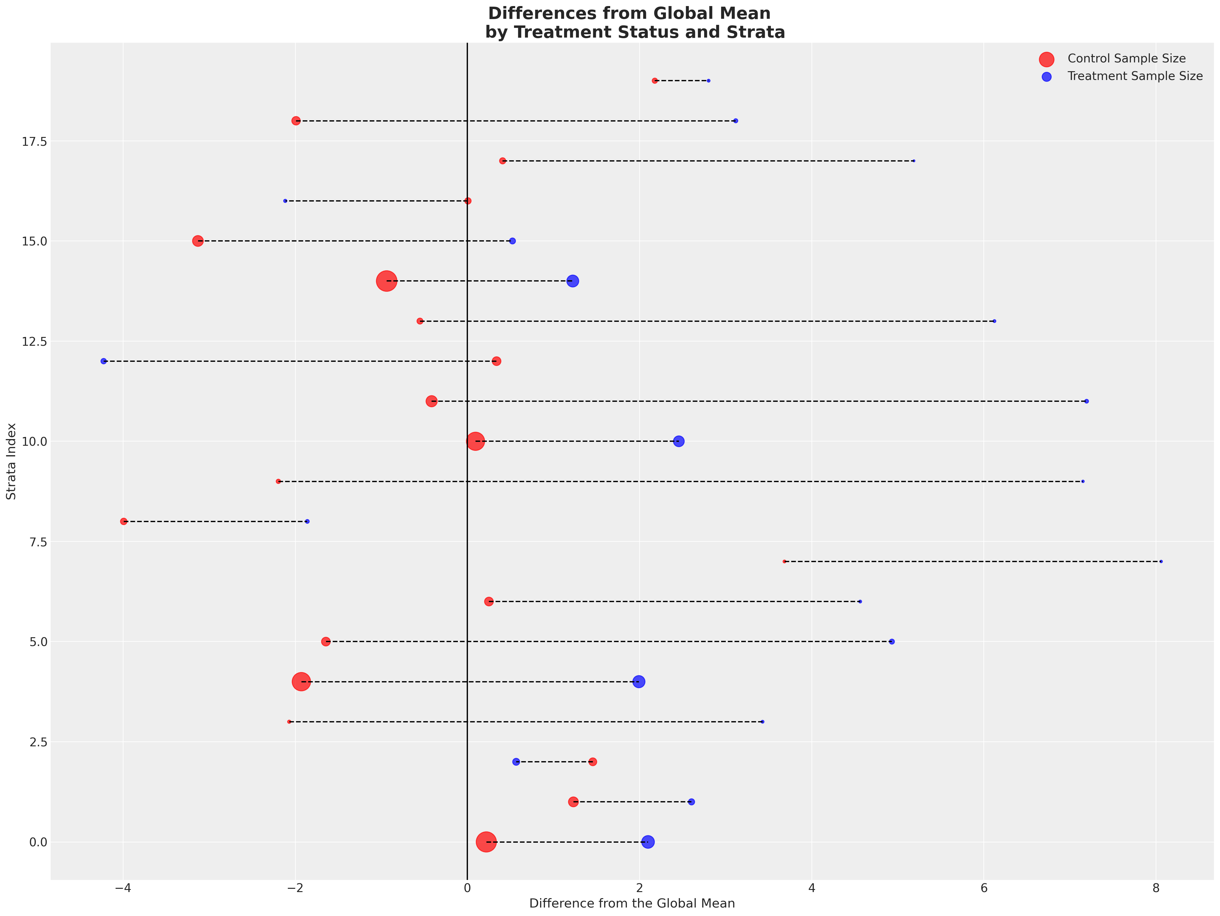
Showing a fairly consistent pattern across the strata - the treatment group achieve outcomes in excess of the global mean almost uniformly across the strata. With smaller sample sizes in each treatment group for each. We then take the average of the stratum specific averages to see a sharper distinction emerge.

strata_expected_df = strata_df.groupby("trt")[["outcome count", "outcome mean", "diff"]].agg(
    {"outcome count": ["sum"], "outcome mean": "mean", "diff": "mean"}
)
print(
    "Treatment Diff:",
    strata_expected_df[("outcome mean", "mean")].iloc[1]
    - strata_expected_df[("outcome mean", "mean")].iloc[0],
)
strata_expected_df

Treatment Diff: 3.662365976037309

	outcome count	outcome mean	diff
	sum	mean	mean
trt
0	1163	1.767384	-0.870916
1	403	5.429750	2.791450

This kind of exercise suggests that the manner in which our sample was constructed i.e. some aspect of the data generating process pulls some strata of the population away from adopting the treatment group and that presence in the treatment group pulls the outcome variable to the right. The propensity for being treated is negatively keyed, so contaminates any causal inference claims. We should be legitimately concerned that failure to account for this kind of bias risks incorrect conclusions about (a) the direction and (b) the degree of effect that quitting has on weight. This is natural in the case of observational studies, we never have random assignment to the treatment condition but modelling the propensity for treatment can help us emulate conditions of random assignment.

Prepare Modelling Data

We now simply prepare the data for modelling in a specific format, removing the outcome and trt from the covariate data X.

X = nhefs_df.copy()
y = nhefs_df["outcome"]
t = nhefs_df["trt"]
X = X.drop(["trt", "outcome"], axis=1)
X.head()

	age	race	sex	smokeintensity	smokeyrs	wt71	active_1	active_2	education_2	education_3	education_4	education_5	exercise_1	exercise_2	age^2	wt71^2	smokeintensity^2	smokeyrs^2
0	42	1	0	30	29	79.04	0	0	0	0	0	0	0	1	1764	6247.3216	900	841
1	36	0	0	20	24	58.63	0	0	1	0	0	0	0	0	1296	3437.4769	400	576
2	56	1	1	20	26	56.81	0	0	1	0	0	0	0	1	3136	3227.3761	400	676
3	68	1	0	3	53	59.42	1	0	0	0	0	0	0	1	4624	3530.7364	9	2809
4	40	0	0	20	19	87.09	1	0	1	0	0	0	1	0	1600	7584.6681	400	361

Propensity Score Modelling

In this first step we define a model building function to capture the probability of treatment i.e. our propensity score for each individual.

We specify two types of model which are to be assessed. One which relies entirely on Logistic regression and another which uses BART (Bayesian Additive Regression Trees) to model the relationships between the covariates and the treatment assignment. The BART model has the benefit of using a tree-based algorithm to explore the interaction effects among the various strata in our sample data. See here for more detail about BART and the PyMC implementation.

Having a flexible model like BART is key to understanding what we are doing when we undertake inverse propensity weighting adjustments. The thought is that any given strata in our dataset will be described by a set of covariates. Types of individual will be represented by these covariate profiles - the attribute vector \(X\). The share of observations within our data which are picked out by any given covariate profile represents a bias towards that type of individual. The modelling of the assignment mechanism with a flexible model like BART allows us to estimate the outcome across a range of strata in our population.

First we model the individual propensity scores as a function of the individual covariate profiles:

def make_propensity_model(X, t, bart=True, probit=True, samples=1000, m=50):
    coords = {"coeffs": list(X.columns), "obs": range(len(X))}
    with pm.Model(coords=coords) as model_ps:
        X_data = pm.MutableData("X", X)
        t_data = pm.MutableData("t", t)
        if bart:
            mu = pmb.BART("mu", X, t, m=m)
            if probit:
                p = pm.Deterministic("p", pm.math.invprobit(mu))
            else:
                p = pm.Deterministic("p", pm.math.invlogit(mu))
        else:
            b = pm.Normal("b", mu=0, sigma=1, dims="coeffs")
            mu = pm.math.dot(X_data, b)
            p = pm.Deterministic("p", pm.math.invlogit(mu))

        t_pred = pm.Bernoulli("t_pred", p=p, observed=t_data, dims="obs")

        idata = pm.sample_prior_predictive()
        idata.extend(pm.sample(samples, random_seed=105, idata_kwargs={"log_likelihood": True}))
        idata.extend(pm.sample_posterior_predictive(idata))
    return model_ps, idata


m_ps_logit, idata_logit = make_propensity_model(X, t, bart=False, samples=1000)

Sampling: [b, t_pred]
Auto-assigning NUTS sampler...
Initializing NUTS using jitter+adapt_diag...
Multiprocess sampling (4 chains in 4 jobs)
NUTS: [b]

100.00% [8000/8000 02:18<00:00 Sampling 4 chains, 0 divergences]

Sampling 4 chains for 1_000 tune and 1_000 draw iterations (4_000 + 4_000 draws total) took 138 seconds.
Sampling: [t_pred]

100.00% [4000/4000 00:00<00:00]

m_ps_probit, idata_probit = make_propensity_model(X, t, bart=True, probit=True, samples=4000)

Sampling: [mu, t_pred]
Multiprocess sampling (4 chains in 4 jobs)
PGBART: [mu]

100.00% [20000/20000 01:48<00:00 Sampling 4 chains, 0 divergences]

Sampling 4 chains for 1_000 tune and 4_000 draw iterations (4_000 + 16_000 draws total) took 109 seconds.
The rhat statistic is larger than 1.01 for some parameters. This indicates problems during sampling. See https://arxiv.org/abs/1903.08008 for details
The effective sample size per chain is smaller than 100 for some parameters.  A higher number is needed for reliable rhat and ess computation. See https://arxiv.org/abs/1903.08008 for details
Sampling: [t_pred]

100.00% [16000/16000 00:01<00:00]

Using Propensity Scores: Weights and Pseudo Populations

Once we have fitted these models we can compare how each model attributes the propensity to treatment (in our case the propensity of quitting) to each and every such measured individual. Let’s plot the distribution of propensity scores for the first 20 or so individuals in the study to see the differences between the two models.

az.plot_forest(
    [idata_logit, idata_probit],
    var_names=["p"],
    coords={"p_dim_0": range(20)},
    figsize=(10, 13),
    combined=True,
    kind="ridgeplot",
    model_names=["Logistic Regression", "BART"],
    r_hat=True,
    ridgeplot_alpha=0.4,
);

These propensity scores can be pulled out and examined alongside the other covariates.

ps_logit = idata_logit["posterior"]["p"].mean(dim=("chain", "draw")).round(2)
ps_logit

<xarray.DataArray 'p' (p_dim_0: 1566)>
array([0.1 , 0.15, 0.13, ..., 0.13, 0.47, 0.18])
Coordinates:
  * p_dim_0  (p_dim_0) int64 0 1 2 3 4 5 6 ... 1560 1561 1562 1563 1564 1565

xarray.DataArray

'p'

• p_dim_0: 1566

• 0.1 0.15 0.13 0.44 0.27 0.16 0.21 ... 0.37 0.13 0.16 0.13 0.47 0.18

  array([0.1 , 0.15, 0.13, ..., 0.13, 0.47, 0.18])

• Coordinates: (1)
  • p_dim_0
    (p_dim_0)
    int64
    0 1 2 3 4 ... 1562 1563 1564 1565

    array([   0,    1,    2, ..., 1563, 1564, 1565])

• Indexes: (1)
  • p_dim_0
    PandasIndex

    PandasIndex(Int64Index([   0,    1,    2,    3,    4,    5,    6,    7,    8,    9,
                ...
                1556, 1557, 1558, 1559, 1560, 1561, 1562, 1563, 1564, 1565],
               dtype='int64', name='p_dim_0', length=1566))

• Attributes: (0)

ps_probit = idata_probit["posterior"]["p"].mean(dim=("chain", "draw")).round(2)
ps_probit

<xarray.DataArray 'p' (p_dim_0: 1566)>
array([0.18, 0.18, 0.17, ..., 0.16, 0.32, 0.28])
Coordinates:
  * p_dim_0  (p_dim_0) int64 0 1 2 3 4 5 6 ... 1560 1561 1562 1563 1564 1565

xarray.DataArray

'p'

• p_dim_0: 1566

• 0.18 0.18 0.17 0.45 0.29 0.25 0.25 ... 0.3 0.19 0.25 0.16 0.32 0.28

  array([0.18, 0.18, 0.17, ..., 0.16, 0.32, 0.28])

• Coordinates: (1)
  • p_dim_0
    (p_dim_0)
    int64
    0 1 2 3 4 ... 1562 1563 1564 1565

    array([   0,    1,    2, ..., 1563, 1564, 1565])

• Indexes: (1)
  • p_dim_0
    PandasIndex

    PandasIndex(Int64Index([   0,    1,    2,    3,    4,    5,    6,    7,    8,    9,
                ...
                1556, 1557, 1558, 1559, 1560, 1561, 1562, 1563, 1564, 1565],
               dtype='int64', name='p_dim_0', length=1566))

• Attributes: (0)

Here we plot the distribution of propensity scores under each model and show how the inverse of the propensity score weights would apply to the observed data points.

Show code cell source Hide code cell source

fig, axs = plt.subplots(3, 2, figsize=(20, 15))
axs = axs.flatten()

colors = {1: "blue", 0: "red"}
axs[0].hist(ps_logit.values[t == 0], ec="black", color="red", bins=30, label="Control", alpha=0.6)
axs[0].hist(
    ps_logit.values[t == 1], ec="black", color="blue", bins=30, label="Treatment", alpha=0.6
)
axs[2].hist(ps_logit.values[t == 0], ec="black", color="red", bins=30, label="Control", alpha=0.6)
axs[2].hist(
    1 - ps_logit.values[t == 1], ec="black", color="blue", bins=30, label="Treatment", alpha=0.6
)
axs[0].set_xlabel("Propensity Scores")
axs[1].set_xlabel("Propensity Scores")
axs[1].set_ylabel("Count of Observations")
axs[0].set_ylabel("Count of Observations")
axs[0].axvline(0.9, color="black", linestyle="--", label="Extreme Propensity Score")
axs[0].axvline(0.1, color="black", linestyle="--")
axs[1].hist(ps_probit.values[t == 0], ec="black", color="red", bins=30, label="Control", alpha=0.6)
axs[1].hist(
    ps_probit.values[t == 1], ec="black", color="blue", bins=30, label="Treatment", alpha=0.6
)
axs[3].hist(ps_probit.values[t == 0], ec="black", color="red", bins=30, label="Control", alpha=0.6)
axs[3].hist(
    1 - ps_probit.values[t == 1], ec="black", color="blue", bins=30, label="Treatment", alpha=0.6
)
axs[3].set_title("Overlap of inverted Propensity Scores")
axs[2].set_title("Overlap of inverted Propensity Scores")
axs[1].axvline(0.9, color="black", linestyle="--", label="Extreme Propensity Score")
axs[1].axvline(0.1, color="black", linestyle="--")
axs[2].axvline(0.9, color="black", linestyle="--", label="Extreme Propensity Score")
axs[2].axvline(0.1, color="black", linestyle="--")
axs[3].axvline(0.9, color="black", linestyle="--", label="Extreme Propensity Score")
axs[3].axvline(0.1, color="black", linestyle="--")
axs[0].set_xlim(0, 1)
axs[1].set_xlim(0, 1)
axs[0].set_title("Propensity Scores under Logistic Regression", fontsize=20)
axs[1].set_title(
    "Propensity Scores under Non-Parametric BART model \n with probit transform", fontsize=20
)
axs[4].scatter(
    X["age"], y, color=t.map(colors), s=(1 / ps_logit.values) * 20, ec="black", alpha=0.4
)
axs[4].set_xlabel("Age")
axs[5].set_xlabel("Age")
axs[5].set_ylabel("y")
axs[4].set_ylabel("y")
axs[4].set_title("Sized by IP Weights")
axs[5].set_title("Sized by IP Weights")
axs[5].scatter(
    X["age"], y, color=t.map(colors), s=(1 / ps_probit.values) * 20, ec="black", alpha=0.4
)
red_patch = mpatches.Patch(color="red", label="Control")
blue_patch = mpatches.Patch(color="blue", label="Treated")
axs[2].legend(handles=[red_patch, blue_patch])
axs[0].legend()
axs[1].legend()
axs[5].legend(handles=[red_patch, blue_patch]);

When we consider the distribution of propensity scores we are looking for positivity i.e. the requirement that the conditional probability of receiving a given treatment cannot be 0 or 1 in any patient subgroup as defined by combinations of covariate values. We do not want to overfit our propensity model and have perfect treatment/control group allocation because that reduces their usefulness in the weighting schemes. The important feature of propensity scores are that they are a measure of similarity across groups - extreme predictions of 0 or 1 would threaten the identifiability of the causal treatment effects. Extreme propensity scores (within a strata defined by some covariate profile) indicate that the model does not believe a causal contrast could be well defined between treatments for those individuals. Or at least, that the sample size of in one of the contrast groups would be extremely small. Some authors recommend drawing a boundary at (.1, .9) to filter out or cap extreme cases to address this kind of overfit, but this is essentially an admission of a mis-specified model.

We can also look at the balance of the covariates across partitions of the propensity score. These kind of plots help us assess the degree to which, conditional on the propensity scores, our sample appears have a balanced profile between the treatment and control groups. We are seeking to show balance of covariate profiles conditional on the propensity score.

Show code cell source Hide code cell source

temp = X.copy()
temp["ps"] = ps_logit.values
temp["ps_cut"] = pd.qcut(temp["ps"], 5)


def plot_balance(temp, col, t):
    fig, axs = plt.subplots(1, 5, figsize=(20, 9))
    axs = axs.flatten()
    for c, ax in zip(np.sort(temp["ps_cut"].unique()), axs):
        std0 = temp[(t == 0) & (temp["ps_cut"] == c)][col].std()
        std1 = temp[(t == 1) & (temp["ps_cut"] == c)][col].std()
        pooled_std = (std0 + std1) / 2
        mean_diff = (
            temp[(t == 0) & (temp["ps_cut"] == c)][col].mean()
            - temp[(t == 1) & (temp["ps_cut"] == c)][col].mean()
        ) / pooled_std
        ax.hist(
            temp[(t == 0) & (temp["ps_cut"] == c)][col],
            alpha=0.6,
            color="red",
            density=True,
            ec="black",
            bins=10,
            cumulative=False,
        )
        ax.hist(
            temp[(t == 1) & (temp["ps_cut"] == c)][col],
            alpha=0.4,
            color="blue",
            density=True,
            ec="black",
            bins=10,
            cumulative=False,
        )
        ax.set_title(f"Propensity Score: {c} \n Standardised Mean Diff {np.round(mean_diff, 4)} ")
        ax.set_xlabel(col)
        red_patch = mpatches.Patch(color="red", label="Control")
        blue_patch = mpatches.Patch(color="blue", label="Treated")
        axs[0].legend(handles=[red_patch, blue_patch])
        plt.suptitle(
            f"Density Functions of {col} \n by Partitions of Propensity Score",
            fontsize=20,
            fontweight="bold",
        )


plot_balance(temp, "age", t)

plot_balance(temp, "wt71", t)

plot_balance(temp, "smokeyrs", t)

plot_balance(temp, "smokeintensity", t)

In an ideal world we would have perfect balance across the treatment groups for each of the covariates, but even approximate balance as we see here is useful. When we have good covariate balance (conditional on the propensity scores) we can then use propensity scores in weighting schemes with models of statistical summaries so as to “correct” the representation of covariate profiles across both groups. If an individual’s propensity score is such that they are highly likely to receive the treatment status e.g .95 then we want to downweight their importance if they occur in the treatment and upweight their importance if they appear in the control group. This makes sense because their high propensity score implies that similar individuals are already heavily present in the treatment group, but less likely to occur in the control group. Hence our corrective strategy to re-weight their contribution to the summary statistics across each group.

Robust and Doubly Robust Weighting Schemes

We’ve been keen to stress that propensity based weights are a corrective. An opportunity for the causal analyst to put their finger on the scale and adjust the representative shares accorded to individuals in the treatment and control groups. Yet, there are no universal correctives, and naturally a variety of alternatives have arisen to fill gaps where simple propensity score weighting fails. We will see below a number of alternative weighting schemes.

The main distinction to call out is between the raw propensity score weights and the doubly-robust theory of propensity score weights.

Doubly robust methods are so named because they represent a compromise estimator for causal effect that combines (i) a treatment assignment model (like propensity scores) and (ii) a more direct response outcome model. The method combines these two estimators in a way to generate a statistically unbiased estimate of the treatment effect. They work well because the way they are combined requires that only one of the models needs to be well-specified. The analyst chooses the components of their weighting scheme in so far as they believe they have correctly modelled either (i) or (ii). This is an interesting tension in the apparent distinction between “design-based” inference and “model-based” inference - the requirement for doubly robust estimators is in a way a concession for the puritanical methodologist; we need both and it’s non-obvious when either will suffice alone.

Estimating Treatment Effects

In this section we build a set of functions to pull out and extract a sample from our posterior distribution of propensity scores; use this propensity score to reweight the observed outcome variable across our treatment and control groups to re-calculate the average treatment effect (ATE). It reweights our data using one of three inverse probability weighting schemes and then plots three views (1) the raw propensity scores across groups (2) the raw outcome distribution and (3) the re-weighted outcome distribution.

First we define a bunch of helper functions for each weighting adjustment method we will explore:

def make_robust_adjustments(X, t):
    X["trt"] = t
    p_of_t = X["trt"].mean()
    X["i_ps"] = np.where(t, (p_of_t / X["ps"]), (1 - p_of_t) / (1 - X["ps"]))
    n_ntrt = X[X["trt"] == 0].shape[0]
    n_trt = X[X["trt"] == 1].shape[0]
    outcome_trt = X[X["trt"] == 1]["outcome"]
    outcome_ntrt = X[X["trt"] == 0]["outcome"]
    i_propensity0 = X[X["trt"] == 0]["i_ps"]
    i_propensity1 = X[X["trt"] == 1]["i_ps"]
    weighted_outcome1 = outcome_trt * i_propensity1
    weighted_outcome0 = outcome_ntrt * i_propensity0
    return weighted_outcome0, weighted_outcome1, n_ntrt, n_trt


def make_raw_adjustments(X, t):
    X["trt"] = t
    X["ps"] = np.where(X["trt"], X["ps"], 1 - X["ps"])
    X["i_ps"] = 1 / X["ps"]
    n_ntrt = n_trt = len(X)
    outcome_trt = X[X["trt"] == 1]["outcome"]
    outcome_ntrt = X[X["trt"] == 0]["outcome"]
    i_propensity0 = X[X["trt"] == 0]["i_ps"]
    i_propensity1 = X[X["trt"] == 1]["i_ps"]
    weighted_outcome1 = outcome_trt * i_propensity1
    weighted_outcome0 = outcome_ntrt * i_propensity0
    return weighted_outcome0, weighted_outcome1, n_ntrt, n_trt


def make_doubly_robust_adjustment(X, t, y):
    m0 = sm.OLS(y[t == 0], X[t == 0].astype(float)).fit()
    m1 = sm.OLS(y[t == 1], X[t == 1].astype(float)).fit()
    m0_pred = m0.predict(X)
    m1_pred = m1.predict(X)
    X["trt"] = t
    X["y"] = y
    ## Compromise between outcome and treatement assignment model
    weighted_outcome0 = (1 - X["trt"]) * (X["y"] - m0_pred) / (1 - X["ps"]) + m0_pred
    weighted_outcome1 = X["trt"] * (X["y"] - m1_pred) / X["ps"] + m1_pred

    return weighted_outcome0, weighted_outcome1, None, None

It’s worth here expanding on the theory of doubly robust estimation. We showed above the code for implementing the compromise between the treatment assignment estimator and the response or outcome estimator. But why is this useful? Consider the functional form of the doubly robust estimator.

\[ \hat{Y(1)} = \frac{1}{n} \sum_{0}^{N} \Bigg[ \frac{T(Y - m_{1}(X))}{p_{T}(X)} + m_{1}(X) \Bigg] \]

\[ \hat{Y(0)} = \frac{1}{n} \sum_{0}^{N} \Bigg[ \frac{(1-T)(Y - m_{0}(X))}{(1-p_{T}(X))} + m_{0}(X) \Bigg] \]

It is not immediately intuitive as to how these formulas effect a compromise between the outcome model and the treatment assignment model. But consider the extreme cases. First imagine our model \(m_{1}\) is a perfect fit to our outcome \(Y\), then the numerator of the fraction is 0 and we end up with an average of the model predictions. Instead imagine model \(m_{1}\) is mis-specified and we have some error \(\epsilon > 0\) in the numerator. If the propensity score model is accurate then in the treated class our denominator should be high… say \(\sim N(.9, .05)\), and as such the estimator adds a number close to \(\epsilon\) back to the \(m_{1}\) prediction. Similar reasoning goes through for the \(Y(0)\) case.

The other estimators are simpler - representing a scaling of the outcome variable by transformations of the estimated propensity scores. Each is an attempt to re-balance the datapoints by what we’ve learned about the propensity for treatment. But the differences in the estimators are (as we’ll see) important in their application.

Now we define the plotting functions for our raw and re-weighted outcomes.

Show code cell source Hide code cell source

def plot_weights(bins, top0, top1, ylim, ax):
    ax.axhline(0, c="gray", linewidth=1)
    ax.set_ylim(ylim)
    bars0 = ax.bar(bins[:-1] + 0.025, top0, width=0.04, facecolor="red", alpha=0.6)
    bars1 = ax.bar(bins[:-1] + 0.025, -top1, width=0.04, facecolor="blue", alpha=0.6)

    for bars in (bars0, bars1):
        for bar in bars:
            bar.set_edgecolor("black")

    for x, y in zip(bins, top0):
        ax.text(x + 0.025, y + 10, str(y), ha="center", va="bottom")

    for x, y in zip(bins, top1):
        ax.text(x + 0.025, -y - 10, str(y), ha="center", va="top")


def make_plot(
    X,
    idata,
    lower_bins=[np.arange(1, 30, 1), np.arange(1, 30, 1)],
    ylims=[
        (-100, 370),
        (
            -40,
            100,
        ),
        (-50, 110),
    ],
    text_pos=(20, 80),
    ps=None,
    method="robust",
):
    X = X.copy()
    if ps is None:
        n_list = list(range(1000))
        ## Choose random ps score from posterior
        choice = np.random.choice(n_list, 1)[0]
        X["ps"] = idata["posterior"]["p"].stack(z=("chain", "draw"))[:, choice].values
    else:
        X["ps"] = ps
    X["trt"] = t
    propensity0 = X[X["trt"] == 0]["ps"]
    propensity1 = X[X["trt"] == 1]["ps"]
    ## Get Weighted Outcomes
    if method == "robust":
        X["outcome"] = y
        weighted_outcome0, weighted_outcome1, n_ntrt, n_trt = make_robust_adjustments(X, t)
    elif method == "raw":
        X["outcome"] = y
        weighted_outcome0, weighted_outcome1, n_ntrt, n_trt = make_raw_adjustments(X, t)
    else:
        weighted_outcome0, weighted_outcome1, _, _ = make_doubly_robust_adjustment(X, t, y)

    ### Top Plot of Propensity Scores
    bins = np.arange(0.025, 0.85, 0.05)
    top0, _ = np.histogram(propensity0, bins=bins)
    top1, _ = np.histogram(propensity1, bins=bins)

    fig, axs = plt.subplots(3, 1, figsize=(20, 20))
    axs = axs.flatten()

    plot_weights(bins, top0, top1, ylims[0], axs[0])
    axs[0].text(0.05, 230, "Control = 0")
    axs[0].text(0.05, -90, "Treatment = 1")

    axs[0].set_ylabel("No. Patients", fontsize=14)
    axs[0].set_xlabel("Estimated Propensity Score", fontsize=14)
    axs[0].set_title(
        "Inferred Propensity Scores and IP Weighted Outcome \n by Treatment and Control",
        fontsize=20,
    )

    ### Middle Plot of Outcome
    outcome_trt = y[t == 1]
    outcome_ntrt = y[t == 0]
    top0, _ = np.histogram(outcome_ntrt, bins=lower_bins[0])
    top1, _ = np.histogram(outcome_trt, bins=lower_bins[0])
    plot_weights(lower_bins[0], top0, top1, ylims[2], axs[1])
    axs[1].set_ylabel("No. Patients", fontsize=14)
    axs[1].set_xlabel("Raw Outcome Measure", fontsize=14)
    axs[1].text(text_pos[0], text_pos[1], f"Control: E(Y) = {outcome_ntrt.mean()}")
    axs[1].text(text_pos[0], text_pos[1] - 20, f"Treatment: E(Y) = {outcome_trt.mean()}")
    axs[1].text(
        text_pos[0],
        text_pos[1] - 40,
        f"tau: E(Y(1) - Y(0)) = {outcome_trt.mean()- outcome_ntrt.mean()}",
        fontweight="bold",
    )

    ## Bottom Plot of Adjusted Outcome using Inverse Propensity Score weights
    axs[2].set_ylabel("No. Patients", fontsize=14)
    if method in ["raw", "robust"]:
        top0, _ = np.histogram(weighted_outcome0, bins=lower_bins[1])
        top1, _ = np.histogram(weighted_outcome1, bins=lower_bins[1])
        plot_weights(lower_bins[1], top0, top1, ylims[1], axs[2])
        axs[2].set_xlabel("Estimated IP Weighted Outcome \n Shifted", fontsize=14)
        axs[2].text(text_pos[0], text_pos[1], f"Control: E(Y) = {weighted_outcome0.sum() / n_ntrt}")
        axs[2].text(
            text_pos[0], text_pos[1] - 20, f"Treatment: E(Y) = {weighted_outcome1.sum() / n_trt}"
        )
        axs[2].text(
            text_pos[0],
            text_pos[1] - 40,
            f"tau: E(Y(1) - Y(0)) = {weighted_outcome1.sum() / n_trt - weighted_outcome0.sum() / n_ntrt}",
            fontweight="bold",
        )
    else:
        top0, _ = np.histogram(weighted_outcome0, bins=lower_bins[1])
        top1, _ = np.histogram(weighted_outcome1, bins=lower_bins[1])
        plot_weights(lower_bins[1], top0, top1, ylims[1], axs[2])
        trt = np.round(np.mean(weighted_outcome1), 5)
        ntrt = np.round(np.mean(weighted_outcome0), 5)
        axs[2].set_xlabel("Estimated IP Weighted Outcome \n Shifted", fontsize=14)
        axs[2].text(text_pos[0], text_pos[1], f"Control: E(Y) = {ntrt}")
        axs[2].text(text_pos[0], text_pos[1] - 20, f"Treatment: E(Y) = {trt}")
        axs[2].text(
            text_pos[0], text_pos[1] - 40, f"tau: E(Y(1) - Y(0)) = {trt - ntrt}", fontweight="bold"
        )

The Logit Propensity Model

We plot the outcome and re-weighted outcome distribution using the robust propensity score estimation method.

make_plot(
    X,
    idata_logit,
    method="robust",
    ps=ps_logit,
    lower_bins=[np.arange(1, 30, 0.5), np.arange(1, 60, 0.5)],
)

There is a lot going on in this plot so it’s worth walking through it a bit more slowly. In the first panel we have the distribution of the propensity scores across both the treatment and control groups. In the second panel we have the raw outcome data plotted again as a distribution split between the groups. Additionally we have presented the expected values of the outcome and the ATE if it were naively estimated on the raw outcome data. Finally on the third panel we have the re-weighted outcome variable - reweighted using the inverse propensity scores, and we derive the ATE based on the adjusted outcome variable. The distinction between the ATE under the raw and adjusted outcome is what we are highlighting in this plot.

Next, and because we are Bayesians - we pull out and evaluate the posterior distribution of the ATE based on the sampled propensity scores. We’ve seen a point estimate for the ATE above, but it’s often more important in the causal inference context to understand the uncertainty in the estimate.

def get_ate(X, t, y, i, idata, method="doubly_robust"):
    X = X.copy()
    X["outcome"] = y
    ### Post processing the sample posterior distribution for propensity scores
    ### One sample at a time.
    X["ps"] = idata["posterior"]["p"].stack(z=("chain", "draw"))[:, i].values
    if method == "robust":
        weighted_outcome_ntrt, weighted_outcome_trt, n_ntrt, n_trt = make_robust_adjustments(X, t)
        ntrt = weighted_outcome_ntrt.sum() / n_ntrt
        trt = weighted_outcome_trt.sum() / n_trt
    elif method == "raw":
        weighted_outcome_ntrt, weighted_outcome_trt, n_ntrt, n_trt = make_raw_adjustments(X, t)
        ntrt = weighted_outcome_ntrt.sum() / n_ntrt
        trt = weighted_outcome_trt.sum() / n_trt
    else:
        X.drop("outcome", axis=1, inplace=True)
        weighted_outcome_ntrt, weighted_outcome_trt, n_ntrt, n_trt = make_doubly_robust_adjustment(
            X, t, y
        )
        trt = np.mean(weighted_outcome_trt)
        ntrt = np.mean(weighted_outcome_ntrt)
    ate = trt - ntrt
    return [ate, trt, ntrt]


qs = range(4000)
ate_dist = [get_ate(X, t, y, q, idata_logit, method="robust") for q in qs]

ate_dist_df_logit = pd.DataFrame(ate_dist, columns=["ATE", "E(Y(1))", "E(Y(0))"])
ate_dist_df_logit.head()

	ATE	E(Y(1))	E(Y(0))
0	3.649712	5.460591	1.810880
1	3.226628	4.998798	1.772170
2	3.700728	5.406525	1.705797
3	3.350942	5.167095	1.816153
4	4.156807	5.784731	1.627924

Next we plot the posterior distribution of the ATE.

Show code cell source Hide code cell source

def plot_ate(ate_dist_df, xy=(4.0, 250)):
    fig, axs = plt.subplots(1, 2, figsize=(20, 7))
    axs = axs.flatten()
    axs[0].hist(
        ate_dist_df["E(Y(1))"], bins=30, ec="black", color="blue", label="E(Y(1))", alpha=0.5
    )
    axs[0].hist(
        ate_dist_df["E(Y(0))"], bins=30, ec="black", color="red", label="E(Y(0))", alpha=0.7
    )
    axs[1].hist(ate_dist_df["ATE"], bins=30, ec="black", color="slateblue", label="ATE", alpha=0.6)
    ate = np.round(ate_dist_df["ATE"].mean(), 2)
    axs[1].axvline(ate, label="E(ATE)", linestyle="--", color="black")
    axs[1].annotate(f"E(ATE): {ate}", xy, fontsize=20, fontweight="bold")
    axs[1].set_title(f"Average Treatment Effect \n E(ATE): {ate}", fontsize=20)
    axs[0].set_title("E(Y) Distributions for Treated and Control", fontsize=20)
    axs[1].set_xlabel("Average Treatment Effect")
    axs[0].set_xlabel("Expected Potential Outcomes")
    axs[1].legend()
    axs[0].legend()


plot_ate(ate_dist_df_logit)

Note how this estimate of the treatment effect is quite different than what we got taking the simple difference of averages across groups.

The BART Propensity Model

Next we’ll apply the raw and then doubly robust estimator to the propensity distribution achieved using the BART non-parametric model.

make_plot(
    X,
    idata_probit,
    method="raw",
    ylims=[(-150, 370), (-220, 150), (-50, 120)],
    lower_bins=[np.arange(1, 30, 0.5), np.arange(1, 60, 0.5)],
)

We see here how the re-weighting scheme for the BART based propensity scores induces a different shape on the outcome distribution than above, but still achieves a similar estimate for the ATE.

ate_dist_probit = [get_ate(X, t, y, q, idata_probit, method="doubly_robust") for q in qs]
ate_dist_df_probit = pd.DataFrame(ate_dist_probit, columns=["ATE", "E(Y(1))", "E(Y(0))"])
ate_dist_df_probit.head()

	ATE	E(Y(1))	E(Y(0))
0	3.304293	5.088071	1.783777
1	3.416959	5.180571	1.763612
2	3.457275	5.229618	1.772343
3	3.531050	5.303977	1.772926
4	3.585944	5.345035	1.759090

plot_ate(ate_dist_df_probit, xy=(3.6, 250))

Note the tighter variance of the measures using the doubly robust method. This is not surprising the doubly robust method was designed with this intended effect.

Considerations when choosing between models

It is one thing to evalute change in average over the population, but we might want to allow for the idea of effect heterogenity across the population and as such the BART model is generally better at ensuring accurate predictions across the deeper strata of our data. But the flexibility of machine learning models for prediction tasks do not guarantee that the propensity scores attributed across the sample are well calibrated to recover the true-treatment effects when used in causal effect estimation. We have to be careful in how we use the flexibility of non-parametric models in the causal context.

First observe the hetereogenous accuracy induced by the BART model across increasingly narrow strata of our sample.

Show code cell source Hide code cell source

fig, axs = plt.subplots(4, 2, figsize=(20, 25))
axs = axs.flatten()
az.plot_ppc(idata_logit, ax=axs[0])
az.plot_ppc(idata_probit, ax=axs[1])
idx1 = list((X[X["race"] == 1].index).values)
idx0 = list((X[X["race"] == 0].index).values)
az.plot_ppc(idata_logit, ax=axs[2], coords={"obs": idx1})
az.plot_ppc(idata_probit, ax=axs[3], coords={"obs": idx0})
idx1 = list((X[(X["race"] == 1) & (X["sex"] == 1)].index).values)
idx0 = list((X[(X["race"] == 0) & (X["sex"] == 1)].index).values)
az.plot_ppc(idata_logit, ax=axs[4], coords={"obs": idx1})
az.plot_ppc(idata_probit, ax=axs[5], coords={"obs": idx0})
idx1 = list((X[(X["race"] == 1) & (X["sex"] == 1) & (X["active_1"] == 1)].index).values)
idx0 = list((X[(X["race"] == 0) & (X["sex"] == 1) & (X["active_1"] == 1)].index).values)
az.plot_ppc(idata_logit, ax=axs[6], coords={"obs": idx1})
az.plot_ppc(idata_probit, ax=axs[7], coords={"obs": idx0})
axs[0].set_title("Overall PPC - Logit")
axs[1].set_title("Overall PPC - BART")
axs[2].set_title("Race Specific PPC - Logit")
axs[3].set_title("Race Specific PPC - BART")
axs[4].set_title("Race/Gender Specific PPC - Logit")
axs[5].set_title("Race/Gender Specific PPC - BART")
axs[6].set_title("Race/Gender/Active Specific PPC - Logit")
axs[7].set_title("Race/Gender/Active Specific PPC - BART")
plt.suptitle("Posterior Predictive Checks - Heterogenous Effects", fontsize=20);

/Users/nathanielforde/mambaforge/envs/pymc_examples_new/lib/python3.9/site-packages/arviz/plots/ppcplot.py:267: FutureWarning: The return type of `Dataset.dims` will be changed to return a set of dimension names in future, in order to be more consistent with `DataArray.dims`. To access a mapping from dimension names to lengths, please use `Dataset.sizes`.
  flatten_pp = list(predictive_dataset.dims.keys())
/Users/nathanielforde/mambaforge/envs/pymc_examples_new/lib/python3.9/site-packages/arviz/plots/ppcplot.py:271: FutureWarning: The return type of `Dataset.dims` will be changed to return a set of dimension names in future, in order to be more consistent with `DataArray.dims`. To access a mapping from dimension names to lengths, please use `Dataset.sizes`.
  flatten = list(observed_data.dims.keys())

Observations like this go a long way to motivating the use of flexible machine learning methods in causal inference. The model used to capture the outcome distribution or the propensity score distribution ought to be sensitive to variation across extremities of the data. We can see above that the predictive power of the simpler logistic regression model deterioriates as we progress down the partitions of the data. We will see an example below where the flexibility of machine learning models such as BART becomes a problem. We’ll also see and how it can be fixed. Paradoxical as it sounds, a more perfect model of the propensity scores will cleanly seperate the treatment classes making re-balancing harder to achieve. In this way, flexible models like BART (which are prone to overfit) need to be used with care in the case of inverse propensity weighting schemes.

Regression with Propensity Scores

Another perhaps more direct method of causal inference is to just use regression analysis. Angrist and Pischke Angrist and Pischke [2008] suggest that the familiar properties of regression make it more desirable, but concede that there is a role for propensity and that the methods can be combined by the cautious analyst. Here we’ll show how we can combine the propensity score in a regression context to derive estimates of treatment effects.

def make_prop_reg_model(X, t, y, idata_ps, covariates=None, samples=1000):
    ### Note the simplication for specifying the mean estimate in the regression
    ### rather than post-processing the whole posterior
    ps = idata_ps["posterior"]["p"].mean(dim=("chain", "draw")).values
    X_temp = pd.DataFrame({"ps": ps, "trt": t, "trt*ps": t * ps})
    if covariates is None:
        X = X_temp
    else:
        X = pd.concat([X_temp, X[covariates]], axis=1)
    coords = {"coeffs": list(X.columns), "obs": range(len(X))}
    with pm.Model(coords=coords) as model_ps_reg:
        sigma = pm.HalfNormal("sigma", 1)
        b = pm.Normal("b", mu=0, sigma=1, dims="coeffs")
        X = pm.MutableData("X", X)
        mu = pm.math.dot(X, b)
        y_pred = pm.Normal("pred", mu, sigma, observed=y, dims="obs")

        idata = pm.sample_prior_predictive()
        idata.extend(pm.sample(samples, idata_kwargs={"log_likelihood": True}))
        idata.extend(pm.sample_posterior_predictive(idata))
    return model_ps_reg, idata


model_ps_reg, idata_ps_reg = make_prop_reg_model(X, t, y, idata_logit)

Sampling: [b, pred, sigma]
Auto-assigning NUTS sampler...
Initializing NUTS using jitter+adapt_diag...
Multiprocess sampling (4 chains in 4 jobs)
NUTS: [sigma, b]

100.00% [8000/8000 00:01<00:00 Sampling 4 chains, 0 divergences]

Sampling 4 chains for 1_000 tune and 1_000 draw iterations (4_000 + 4_000 draws total) took 1 seconds.
Sampling: [pred]

100.00% [4000/4000 00:00<00:00]

Fitting the regression model using the propensity score as a dimensional reduction technique seems to work well here. We recover substantially the same treatment effect estimate as above.

az.summary(idata_ps_reg)

	mean	sd	hdi_3%	hdi_97%	mcse_mean	mcse_sd	ess_bulk	ess_tail	r_hat
b[ps]	2.450	0.614	1.330	3.663	0.010	0.007	3484.0	3083.0	1.0
b[trt]	3.473	0.482	2.575	4.376	0.009	0.006	2829.0	2664.0	1.0
b[trt*ps]	-0.727	0.959	-2.517	1.121	0.018	0.014	2900.0	2726.0	1.0
sigma	7.806	0.137	7.542	8.061	0.002	0.002	4139.0	2668.0	1.0

model_ps_reg_bart, idata_ps_reg_bart = make_prop_reg_model(X, t, y, idata_probit)

Sampling: [b, pred, sigma]
Auto-assigning NUTS sampler...
Initializing NUTS using jitter+adapt_diag...
Multiprocess sampling (4 chains in 4 jobs)
NUTS: [sigma, b]

100.00% [8000/8000 00:01<00:00 Sampling 4 chains, 0 divergences]

Sampling 4 chains for 1_000 tune and 1_000 draw iterations (4_000 + 4_000 draws total) took 1 seconds.
Sampling: [pred]

100.00% [4000/4000 00:00<00:00]

az.summary(idata_ps_reg_bart)

	mean	sd	hdi_3%	hdi_97%	mcse_mean	mcse_sd	ess_bulk	ess_tail	r_hat
b[ps]	3.228	0.663	1.973	4.460	0.011	0.008	3568.0	2967.0	1.0
b[trt]	3.162	0.470	2.306	4.069	0.009	0.006	2859.0	2467.0	1.0
b[trt*ps]	-0.301	0.954	-2.038	1.554	0.017	0.013	3329.0	3087.0	1.0
sigma	7.780	0.133	7.532	8.028	0.002	0.001	4052.0	2978.0	1.0

Causal Inference as Regression Imputation

Above we read-off the causal effect estimate as the coefficient on the treatment variable in our regression model. An arguably cleaner approach uses the fitted regression models to impute the distribution of potential outcomes Y(1), Y(0) under different treatment regimes. In this way we have yet another perspective on causal inference. Crucially this perspective is non-parametric in that it does not make any assumptions about the required functional form of the imputation models.

X_mod = X.copy()
X_mod["ps"] = ps = idata_probit["posterior"]["p"].mean(dim=("chain", "draw")).values
X_mod["trt"] = 1
X_mod["trt*ps"] = X_mod["ps"] * X_mod["trt"]
with model_ps_reg_bart:
    # update values of predictors:
    pm.set_data({"X": X_mod[["ps", "trt", "trt*ps"]]})
    idata_trt = pm.sample_posterior_predictive(idata_ps_reg_bart)

idata_trt

Sampling: [pred]

100.00% [4000/4000 00:00<00:00]

arviz.InferenceData

• posterior_predictive

  <xarray.Dataset>
  Dimensions:  (chain: 4, draw: 1000, obs: 1566)
  Coordinates:
    * chain    (chain) int64 0 1 2 3
    * draw     (draw) int64 0 1 2 3 4 5 6 7 8 ... 992 993 994 995 996 997 998 999
    * obs      (obs) int64 0 1 2 3 4 5 6 7 ... 1559 1560 1561 1562 1563 1564 1565
  Data variables:
      pred     (chain, draw, obs) float64 -0.7491 0.1096 15.44 ... 3.267 0.2888
  Attributes:
      created_at:                 2024-02-24T19:03:12.138120
      arviz_version:              0.17.0
      inference_library:          pymc
      inference_library_version:  5.3.0

  xarray.Dataset

  • Dimensions:
    • chain: 4
    • draw: 1000
    • obs: 1566
  • Coordinates: (3)
    • chain
      (chain)
      int64
      0 1 2 3

      array([0, 1, 2, 3])

    • draw
      (draw)
      int64
      0 1 2 3 4 5 ... 995 996 997 998 999

      array([  0,   1,   2, ..., 997, 998, 999])

    • obs
      (obs)
      int64
      0 1 2 3 4 ... 1562 1563 1564 1565

      array([   0,    1,    2, ..., 1563, 1564, 1565])

  • Data variables: (1)
    • pred
      (chain, draw, obs)
      float64
      -0.7491 0.1096 ... 3.267 0.2888

      array([[[ -0.7491322 ,   0.10957889,  15.44281264, ...,   5.82599984,
                 1.82004731,   4.33330679],
              [  8.25973555,   7.11144384,   8.99497342, ...,  -4.09511343,
                 9.38524586,  11.71975368],
              [ 10.11359596,   8.81767687,   0.51217981, ...,  -1.08245341,
                 5.84310127,  -9.66342007],
              ...,
              [ 11.49295539,  -3.26130618,  -5.20479679, ...,   5.36998491,
                -0.11324963,   6.3135136 ],
              [ 11.20341739,  17.12532856,  10.82804086, ...,  -5.38384927,
                 1.32969545, -21.71500963],
              [  0.25804463, -10.77536708,   6.97958432, ...,   7.18589735,
                10.74965183,  -0.70316906]],
      
             [[  2.92748462,  13.14121213,  -5.06255015, ...,   6.80282222,
                -6.51186673,  15.77505285],
              [-11.64428595,  10.19830118,   8.96104053, ...,   1.51486588,
                 6.48074076,  13.2031975 ],
              [  0.93901594,  16.1219016 ,   5.18976312, ...,   2.06416863,
                10.25523995,  -0.79588665],
      ...
              [  5.21970117,   3.48032127,   4.76479987, ..., -10.45978891,
                 1.34108776,   7.05721426],
              [ 16.74487971,   0.82852686,   5.00785826, ...,   4.9554557 ,
                 4.022945  ,   8.21547017],
              [ -5.43682812,   9.19418962,  12.03472603, ...,   3.26663288,
                -0.6925452 ,  -3.40710025]],
      
             [[ -2.81199412,   4.80013059,   7.22207454, ...,   6.01629213,
                 3.80815641,  14.4183844 ],
              [ -3.21761143,  12.99047678,   9.1708461 , ...,   8.5547272 ,
                 2.48093278,  -7.180272  ],
              [ 12.80818977,  -1.72298684,  10.2833022 , ...,   6.99822141,
                 4.86439872,   4.98314346],
              ...,
              [ 11.05884019,  -2.16453136,   3.96512699, ...,   5.86510329,
                 1.09121914,   4.65136986],
              [  1.8813462 ,   6.33468741,   6.69923338, ...,  11.37401696,
                 0.15886388,   6.54986507],
              [ 12.14495678,  -0.26719089,   9.43889935, ...,  -2.65620619,
                 3.26736877,   0.28884295]]])

  • Indexes: (3)
    • chain
      PandasIndex

      PandasIndex(Int64Index([0, 1, 2, 3], dtype='int64', name='chain'))

    • draw
      PandasIndex

      PandasIndex(Int64Index([  0,   1,   2,   3,   4,   5,   6,   7,   8,   9,
                  ...
                  990, 991, 992, 993, 994, 995, 996, 997, 998, 999],
                 dtype='int64', name='draw', length=1000))

    • obs
      PandasIndex

      PandasIndex(Int64Index([   0,    1,    2,    3,    4,    5,    6,    7,    8,    9,
                  ...
                  1556, 1557, 1558, 1559, 1560, 1561, 1562, 1563, 1564, 1565],
                 dtype='int64', name='obs', length=1566))

  • Attributes: (4)

    created_at :

    2024-02-24T19:03:12.138120

    arviz_version :

    0.17.0

    inference_library :

    pymc

    inference_library_version :

    5.3.0

  
  
• observed_data

  <xarray.Dataset>
  Dimensions:  (obs: 1566)
  Coordinates:
    * obs      (obs) int64 0 1 2 3 4 5 6 7 ... 1559 1560 1561 1562 1563 1564 1565
  Data variables:
      pred     (obs) float64 -10.09 2.605 9.414 4.99 ... 1.36 3.515 4.763 15.76
  Attributes:
      created_at:                 2024-02-24T19:03:12.139483
      arviz_version:              0.17.0
      inference_library:          pymc
      inference_library_version:  5.3.0

  xarray.Dataset

  • Dimensions:
    • obs: 1566
  • Coordinates: (1)
    • obs
      (obs)
      int64
      0 1 2 3 4 ... 1562 1563 1564 1565

      array([   0,    1,    2, ..., 1563, 1564, 1565])

  • Data variables: (1)
    • pred
      (obs)
      float64
      -10.09 2.605 9.414 ... 4.763 15.76

      array([-10.09395976,   2.60496995,   9.41448602, ...,   3.51496995,
               4.76263862,  15.76420695])

  • Indexes: (1)
    • obs
      PandasIndex

      PandasIndex(Int64Index([   0,    1,    2,    3,    4,    5,    6,    7,    8,    9,
                  ...
                  1556, 1557, 1558, 1559, 1560, 1561, 1562, 1563, 1564, 1565],
                 dtype='int64', name='obs', length=1566))

  • Attributes: (4)

    created_at :

    2024-02-24T19:03:12.139483

    arviz_version :

    0.17.0

    inference_library :

    pymc

    inference_library_version :

    5.3.0

  
  
• constant_data

  <xarray.Dataset>
  Dimensions:  (X_dim_0: 1566, X_dim_1: 3)
  Coordinates:
    * X_dim_0  (X_dim_0) int64 0 1 2 3 4 5 6 ... 1560 1561 1562 1563 1564 1565
    * X_dim_1  (X_dim_1) int64 0 1 2
  Data variables:
      X        (X_dim_0, X_dim_1) float64 0.1815 1.0 0.1815 ... 0.2776 1.0 0.2776
  Attributes:
      created_at:                 2024-02-24T19:03:12.140418
      arviz_version:              0.17.0
      inference_library:          pymc
      inference_library_version:  5.3.0

  xarray.Dataset

  • Dimensions:
    • X_dim_0: 1566
    • X_dim_1: 3
  • Coordinates: (2)
    • X_dim_0
      (X_dim_0)
      int64
      0 1 2 3 4 ... 1562 1563 1564 1565

      array([   0,    1,    2, ..., 1563, 1564, 1565])

    • X_dim_1
      (X_dim_1)
      int64
      0 1 2

      array([0, 1, 2])

  • Data variables: (1)
    • X
      (X_dim_0, X_dim_1)
      float64
      0.1815 1.0 0.1815 ... 1.0 0.2776

      array([[0.18145026, 1.        , 0.18145026],
             [0.17577815, 1.        , 0.17577815],
             [0.17011745, 1.        , 0.17011745],
             ...,
             [0.15631114, 1.        , 0.15631114],
             [0.32063229, 1.        , 0.32063229],
             [0.2775787 , 1.        , 0.2775787 ]])

  • Indexes: (2)
    • X_dim_0
      PandasIndex

      PandasIndex(Int64Index([   0,    1,    2,    3,    4,    5,    6,    7,    8,    9,
                  ...
                  1556, 1557, 1558, 1559, 1560, 1561, 1562, 1563, 1564, 1565],
                 dtype='int64', name='X_dim_0', length=1566))

    • X_dim_1
      PandasIndex

      PandasIndex(Int64Index([0, 1, 2], dtype='int64', name='X_dim_1'))

  • Attributes: (4)

    created_at :

    2024-02-24T19:03:12.140418

    arviz_version :

    0.17.0

    inference_library :

    pymc

    inference_library_version :

    5.3.0

  
  

X_mod = X.copy()
X_mod["ps"] = ps = idata_probit["posterior"]["p"].mean(dim=("chain", "draw")).values
X_mod["trt"] = 0
X_mod["trt*ps"] = X_mod["ps"] * X_mod["trt"]
with model_ps_reg_bart:
    # update values of predictors:
    pm.set_data({"X": X_mod[["ps", "trt", "trt*ps"]]})
    idata_ntrt = pm.sample_posterior_predictive(idata_ps_reg_bart)

idata_ntrt

Sampling: [pred]

100.00% [4000/4000 00:00<00:00]

arviz.InferenceData

• posterior_predictive

  <xarray.Dataset>
  Dimensions:  (chain: 4, draw: 1000, obs: 1566)
  Coordinates:
    * chain    (chain) int64 0 1 2 3
    * draw     (draw) int64 0 1 2 3 4 5 6 7 8 ... 992 993 994 995 996 997 998 999
    * obs      (obs) int64 0 1 2 3 4 5 6 7 ... 1559 1560 1561 1562 1563 1564 1565
  Data variables:
      pred     (chain, draw, obs) float64 -13.99 5.743 -3.888 ... 3.793 -2.711
  Attributes:
      created_at:                 2024-02-24T19:03:12.404939
      arviz_version:              0.17.0
      inference_library:          pymc
      inference_library_version:  5.3.0

  xarray.Dataset

  • Dimensions:
    • chain: 4
    • draw: 1000
    • obs: 1566
  • Coordinates: (3)
    • chain
      (chain)
      int64
      0 1 2 3

      array([0, 1, 2, 3])

    • draw
      (draw)
      int64
      0 1 2 3 4 5 ... 995 996 997 998 999

      array([  0,   1,   2, ..., 997, 998, 999])

    • obs
      (obs)
      int64
      0 1 2 3 4 ... 1562 1563 1564 1565

      array([   0,    1,    2, ..., 1563, 1564, 1565])

  • Data variables: (1)
    • pred
      (chain, draw, obs)
      float64
      -13.99 5.743 ... 3.793 -2.711

      array([[[-13.9857916 ,   5.74328033,  -3.88835993, ...,   9.28556655,
                -2.84309099,   1.74638744],
              [  5.95033082,   5.6946622 ,   1.1467397 , ...,   9.49259481,
                 7.02797621,  -7.77014893],
              [-14.87364941,   6.32954459,  -1.03913643, ...,   7.79034807,
                -0.15273026,  -6.24600659],
              ...,
              [-11.58578887, -18.40978016,   9.57362455, ...,   7.43967708,
                 7.83957617,  -3.58747471],
              [ -4.00305168,  10.77220155,  -1.22917474, ...,   3.45231689,
                 8.32167264,   4.77612768],
              [  3.96655997,   1.17330818,   8.34549976, ...,  -4.0340873 ,
                 7.71253378,  17.81151361]],
      
             [[  2.54600776,  -3.68070811,  -1.55178351, ...,   0.50694488,
                -0.84032035,  -9.42068662],
              [  6.07591768,  -2.01446835,  -2.82993283, ...,   6.91178834,
                 0.25150675,   7.76991278],
              [  6.43978322,  -2.26215117,   7.79623406, ...,  -3.22651403,
                 2.35078511,   9.34859133],
      ...
              [ -3.65358817,   6.100932  ,  24.06746093, ...,  13.58662259,
                10.98339339,   4.74411048],
              [ -8.85114866,  -0.18792118,   4.00662137, ...,  -4.9914739 ,
                -3.82746867,  -5.50923469],
              [ -2.55398859,  -1.37022197,  -5.61381551, ...,  -2.95534869,
                13.77576083,  -2.23551625]],
      
             [[  2.74520922,  -0.51970556,   5.67230597, ..., -11.25743125,
                -0.11912179,  16.47656619],
              [-10.71666659,  -9.26042498,   0.76178451, ..., -10.90878026,
                 6.45285949,  13.67479583],
              [ -0.27296419,  -0.50940722,  -0.23164144, ...,   0.0664804 ,
                 9.03494895,  12.49568519],
              ...,
              [ 17.39120023,  -9.83677991,  -1.95375499, ...,   0.69160671,
                -5.43936128,  -3.56630278],
              [ -1.65464033,  -6.58515835,  11.11668412, ...,  -9.90863731,
                -6.41945429,   8.1475955 ],
              [ -1.17304069,   9.23961933,  -7.62247269, ...,  -2.93939843,
                 3.79278769,  -2.7105666 ]]])

  • Indexes: (3)
    • chain
      PandasIndex

      PandasIndex(Int64Index([0, 1, 2, 3], dtype='int64', name='chain'))

    • draw
      PandasIndex

      PandasIndex(Int64Index([  0,   1,   2,   3,   4,   5,   6,   7,   8,   9,
                  ...
                  990, 991, 992, 993, 994, 995, 996, 997, 998, 999],
                 dtype='int64', name='draw', length=1000))

    • obs
      PandasIndex

      PandasIndex(Int64Index([   0,    1,    2,    3,    4,    5,    6,    7,    8,    9,
                  ...
                  1556, 1557, 1558, 1559, 1560, 1561, 1562, 1563, 1564, 1565],
                 dtype='int64', name='obs', length=1566))

  • Attributes: (4)

    created_at :

    2024-02-24T19:03:12.404939

    arviz_version :

    0.17.0

    inference_library :

    pymc

    inference_library_version :

    5.3.0

  
  
• observed_data

  <xarray.Dataset>
  Dimensions:  (obs: 1566)
  Coordinates:
    * obs      (obs) int64 0 1 2 3 4 5 6 7 ... 1559 1560 1561 1562 1563 1564 1565
  Data variables:
      pred     (obs) float64 -10.09 2.605 9.414 4.99 ... 1.36 3.515 4.763 15.76
  Attributes:
      created_at:                 2024-02-24T19:03:12.406164
      arviz_version:              0.17.0
      inference_library:          pymc
      inference_library_version:  5.3.0

  xarray.Dataset

  • Dimensions:
    • obs: 1566
  • Coordinates: (1)
    • obs
      (obs)
      int64
      0 1 2 3 4 ... 1562 1563 1564 1565

      array([   0,    1,    2, ..., 1563, 1564, 1565])

  • Data variables: (1)
    • pred
      (obs)
      float64
      -10.09 2.605 9.414 ... 4.763 15.76

      array([-10.09395976,   2.60496995,   9.41448602, ...,   3.51496995,
               4.76263862,  15.76420695])

  • Indexes: (1)
    • obs
      PandasIndex

      PandasIndex(Int64Index([   0,    1,    2,    3,    4,    5,    6,    7,    8,    9,
                  ...
                  1556, 1557, 1558, 1559, 1560, 1561, 1562, 1563, 1564, 1565],
                 dtype='int64', name='obs', length=1566))

  • Attributes: (4)

    created_at :

    2024-02-24T19:03:12.406164

    arviz_version :

    0.17.0

    inference_library :

    pymc

    inference_library_version :

    5.3.0

  
  
• constant_data

  <xarray.Dataset>
  Dimensions:  (X_dim_0: 1566, X_dim_1: 3)
  Coordinates:
    * X_dim_0  (X_dim_0) int64 0 1 2 3 4 5 6 ... 1560 1561 1562 1563 1564 1565
    * X_dim_1  (X_dim_1) int64 0 1 2
  Data variables:
      X        (X_dim_0, X_dim_1) float64 0.1815 0.0 0.0 0.1758 ... 0.2776 0.0 0.0
  Attributes:
      created_at:                 2024-02-24T19:03:12.407083
      arviz_version:              0.17.0
      inference_library:          pymc
      inference_library_version:  5.3.0

  xarray.Dataset

  • Dimensions:
    • X_dim_0: 1566
    • X_dim_1: 3
  • Coordinates: (2)
    • X_dim_0
      (X_dim_0)
      int64
      0 1 2 3 4 ... 1562 1563 1564 1565

      array([   0,    1,    2, ..., 1563, 1564, 1565])

    • X_dim_1
      (X_dim_1)
      int64
      0 1 2

      array([0, 1, 2])

  • Data variables: (1)
    • X
      (X_dim_0, X_dim_1)
      float64
      0.1815 0.0 0.0 ... 0.2776 0.0 0.0

      array([[0.18145026, 0.        , 0.        ],
             [0.17577815, 0.        , 0.        ],
             [0.17011745, 0.        , 0.        ],
             ...,
             [0.15631114, 0.        , 0.        ],
             [0.32063229, 0.        , 0.        ],
             [0.2775787 , 0.        , 0.        ]])

  • Indexes: (2)
    • X_dim_0
      PandasIndex

      PandasIndex(Int64Index([   0,    1,    2,    3,    4,    5,    6,    7,    8,    9,
                  ...
                  1556, 1557, 1558, 1559, 1560, 1561, 1562, 1563, 1564, 1565],
                 dtype='int64', name='X_dim_0', length=1566))

    • X_dim_1
      PandasIndex

      PandasIndex(Int64Index([0, 1, 2], dtype='int64', name='X_dim_1'))

  • Attributes: (4)

    created_at :

    2024-02-24T19:03:12.407083

    arviz_version :

    0.17.0

    inference_library :

    pymc

    inference_library_version :

    5.3.0

  
  

idata_trt["posterior_predictive"]["pred"].mean()

<xarray.DataArray 'pred' ()>
array(3.91691031)

xarray.DataArray

'pred'

• 3.917

  array(3.91691031)

• Coordinates: (0)
• Indexes: (0)
• Attributes: (0)

idata_ntrt["posterior_predictive"]["pred"].mean()

<xarray.DataArray 'pred' ()>
array(0.82496553)

xarray.DataArray

'pred'

• 0.825

  array(0.82496553)

• Coordinates: (0)
• Indexes: (0)
• Attributes: (0)

idata_trt["posterior_predictive"]["pred"].mean() - idata_ntrt["posterior_predictive"]["pred"].mean()

<xarray.DataArray 'pred' ()>
array(3.09194478)

xarray.DataArray

'pred'

• 3.092

  array(3.09194478)

• Coordinates: (0)
• Indexes: (0)
• Attributes: (0)

All these perspectives on the question of causal inference here seem broadly convergent. Next we’ll see an example where the choices an analyst makes can go quite wrong and real care needs to be made in the application of these inferential tools.

Confounded Inference: Health Expenditure Data

We will now begin with looking at a health-expenditure data set analysed in Bayesian Nonparametrics for Causal Inference and Missing Data . The telling feature about this data set is the absence of obvious causal impact on expenditure due to the presence of smoking. We follow the authors and try and model the effect of smoke on the logged out log_y. We’ll focus initially on estimating the ATE. There is little signal to discern regarding the effects of smoking. We want to demonstrate how even if we choose the right methods and try to control for bias with the right tools - we can miss the story under our nose if we’re too focused on the mechanics and not the data generating process.

try:
    df = pd.read_csv("../data/meps_bayes_np_health.csv", index_col=["Unnamed: 0"])
except:
    df = pd.read_csv(pm.get_data("meps_bayes_np_health.csv"), index_col=["Unnamed: 0"])

df = df[df["totexp"] > 0].reset_index(drop=True)
df["log_y"] = np.log(df["totexp"] + 1000)
df["loginc"] = np.log(df["income"])
df["smoke"] = np.where(df["smoke"] == "No", 0, 1)
df

/Users/nathanielforde/mambaforge/envs/pymc_examples_new/lib/python3.9/site-packages/pandas/core/arraylike.py:402: RuntimeWarning: divide by zero encountered in log
  result = getattr(ufunc, method)(*inputs, **kwargs)

	age	bmi	edu	income	povlev	region	sex	marital	race	seatbelt	smoke	phealth	totexp	log_y	loginc
0	30	39.1	14	78400	343.69	Northeast	Male	Married	White	Always	0	Fair	40	6.946976	11.269579
1	53	20.2	17	180932	999.30	West	Male	Married	Multi	Always	0	Very Good	429	7.264730	12.105877
2	81	21.0	14	27999	205.94	West	Male	Married	White	Always	0	Very Good	14285	9.634627	10.239924
3	77	25.7	12	27999	205.94	West	Female	Married	White	Always	0	Fair	7959	9.100414	10.239924
4	31	23.0	12	14800	95.46	South	Female	Divorced	White	Always	0	Excellent	5017	8.702344	9.602382
...	...	...	...	...	...	...	...	...	...	...	...	...	...	...	...
16425	23	26.6	16	23000	130.72	South	Male	Separated	Asian	Always	0	Very Good	130	7.029973	10.043249
16426	55	21.9	12	23000	130.72	South	Female	Married	Asian	Always	0	Very Good	468	7.291656	10.043249
16427	22	-9.0	9	7000	38.66	Midwest	Male	Married	White	Always	0	Excellent	711	7.444833	8.853665
16428	22	24.2	10	7000	38.66	Midwest	Female	Married	White	Always	0	Excellent	587	7.369601	8.853665
16429	20	26.9	10	9858	84.24	Midwest	Female	Separated	White	Always	0	Fair	1228	7.708860	9.196039

16430 rows × 15 columns

Summary Statistics

Lets review the basic summary statistics and see how they change across various strata of the population

raw_diff = df.groupby("smoke")[["log_y"]].mean()
print("Treatment Diff:", raw_diff["log_y"].iloc[0] - raw_diff["log_y"].iloc[1])
raw_diff

Treatment Diff: 0.05280094075302166

	log_y
smoke
0	8.098114
1	8.045313

pd.set_option("display.max_rows", 500)
strata_df = df.groupby(["smoke", "sex", "race", "phealth"])[["log_y"]].agg(["count", "mean", "std"])

global_avg = df["log_y"].mean()
strata_df["global_avg"] = global_avg
strata_df.reset_index(inplace=True)
strata_df.columns = [" ".join(col).strip() for col in strata_df.columns.values]
strata_df["diff"] = strata_df["log_y mean"] - strata_df["global_avg"]
strata_df.sort_values("log_y count", ascending=False).head(30).style.background_gradient(axis=0)

	smoke	sex	race	phealth	log_y count	log_y mean	log_y std	global_avg	diff
29	0	Female	White	Very Good	1858	8.101406	0.896128	8.089203	0.012204
27	0	Female	White	Good	1572	8.231117	1.010783	8.089203	0.141914
25	0	Female	White	Excellent	1385	7.919802	0.846725	8.089203	-0.169400
59	0	Male	White	Very Good	1321	7.987652	0.922520	8.089203	-0.101551
57	0	Male	White	Good	1129	8.178290	1.003363	8.089203	0.089088
55	0	Male	White	Excellent	1122	7.728966	0.779346	8.089203	-0.360236
26	0	Female	White	Fair	659	8.487774	1.113656	8.089203	0.398572
7	0	Female	Black	Good	515	8.125243	0.944796	8.089203	0.036040
9	0	Female	Black	Very Good	488	7.870293	0.884956	8.089203	-0.218909
56	0	Male	White	Fair	434	8.601018	1.112748	8.089203	0.511816
110	1	Male	White	Good	335	7.939632	0.887826	8.089203	-0.149571
84	1	Female	White	Good	324	8.077777	0.968686	8.089203	-0.011426
5	0	Female	Black	Excellent	307	7.748597	0.812461	8.089203	-0.340606
6	0	Female	Black	Fair	266	8.534893	1.057159	8.089203	0.445690
86	1	Female	White	Very Good	266	7.913179	0.902211	8.089203	-0.176024
39	0	Male	Black	Very Good	246	7.765843	0.831623	8.089203	-0.323360
37	0	Male	Black	Good	235	8.002760	1.051284	8.089203	-0.086443
112	1	Male	White	Very Good	235	7.848349	0.900002	8.089203	-0.240854
4	0	Female	Asian	Very Good	193	7.864920	0.859187	8.089203	-0.224283
83	1	Female	White	Fair	191	8.403307	0.989581	8.089203	0.314105
28	0	Female	White	Poor	186	9.160054	1.138894	8.089203	1.070852
35	0	Male	Black	Excellent	184	7.620076	0.771911	8.089203	-0.469127
0	0	Female	Asian	Excellent	164	7.786508	0.899504	8.089203	-0.302694
2	0	Female	Asian	Good	162	7.873122	0.768487	8.089203	-0.216080
82	1	Female	White	Excellent	149	7.860320	0.837483	8.089203	-0.228882
108	1	Male	White	Excellent	148	7.652529	0.717871	8.089203	-0.436674
109	1	Male	White	Fair	148	8.282303	1.111403	8.089203	0.193101
58	0	Male	White	Poor	140	9.308711	1.255442	8.089203	1.219509
34	0	Male	Asian	Very Good	140	7.792831	0.772666	8.089203	-0.296371
32	0	Male	Asian	Good	134	7.993583	1.123291	8.089203	-0.095620

Show code cell source Hide code cell source

def make_strata_plot(strata_df):
    joined_df = strata_df[strata_df["smoke"] == 0].merge(
        strata_df[strata_df["smoke"] == 1], on=["sex", "race", "phealth"]
    )
    joined_df.sort_values("diff_y", inplace=True)

    # Func to draw line segment
    def newline(p1, p2, color="black"):
        ax = plt.gca()
        l = mlines.Line2D([p1[0], p2[0]], [p1[1], p2[1]], color="black", linestyle="--")
        ax.add_line(l)
        return l

    fig, ax = plt.subplots(figsize=(20, 15))

    ax.scatter(
        joined_df["diff_x"],
        joined_df.index,
        color="red",
        alpha=0.7,
        label="Control Sample Size",
        s=joined_df["log_y count_x"] / 2,
    )
    ax.scatter(
        joined_df["diff_y"],
        joined_df.index,
        color="blue",
        alpha=0.7,
        label="Treatment Sample Size",
        s=joined_df["log_y count_y"] / 2,
    )

    for i, p1, p2 in zip(joined_df.index, joined_df["diff_x"], joined_df["diff_y"]):
        newline([p1, i], [p2, i])

    ax.set_xlabel("Difference from the Global Mean")
    ax.set_title(
        "Differences from Global Mean \n by Treatment Status and Strata",
        fontsize=20,
        fontweight="bold",
    )
    ax.axvline(0, color="k")
    ax.set_ylabel("Strata Index")
    ax.legend()


make_strata_plot(strata_df)

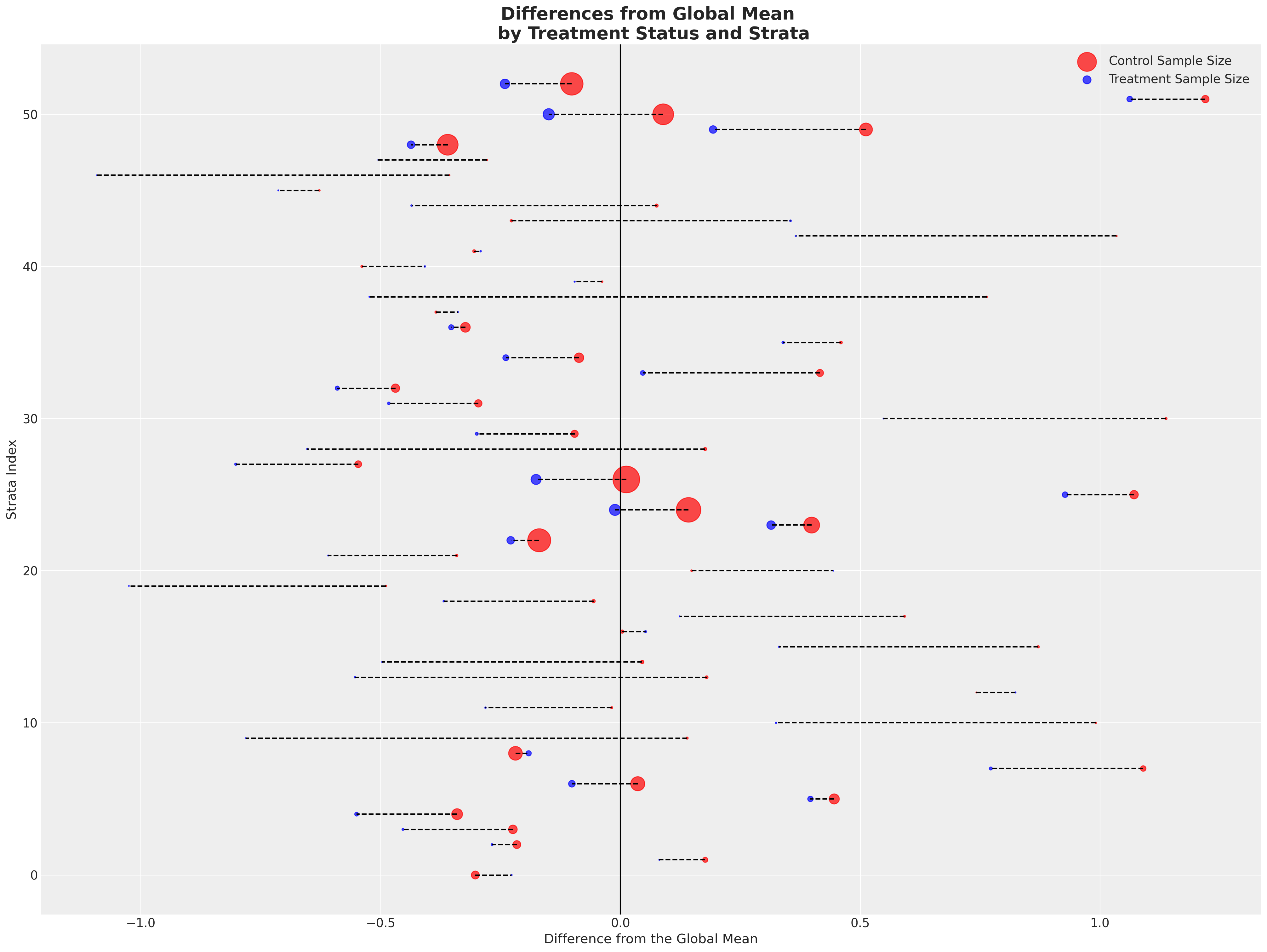
It’s difficult to see a clear pattern in this visual. In both treatment groups, when there is some significant sample size, we see a mean difference close to zero for both groups.

strata_expected_df = strata_df.groupby("smoke")[["log_y count", "log_y mean", "diff"]].agg(
    {"log_y count": ["sum"], "log_y mean": "mean", "diff": "mean"}
)
print(
    "Treatment Diff:",
    strata_expected_df[("log_y mean", "mean")].iloc[0]
    - strata_expected_df[("log_y mean", "mean")].iloc[1],
)
strata_expected_df

Treatment Diff: 0.28947855780477827

	log_y count	log_y mean	diff
	sum	mean	mean
smoke
0	13657	8.237595	0.148392
1	2773	7.948116	-0.141087

It certainly seems that there is little to no impact due to our treatment effect in the data. Can we recover this insight using the method of inverse propensity score weighting?

fig, axs = plt.subplots(2, 2, figsize=(20, 8))
axs = axs.flatten()
axs[0].hist(
    df[df["smoke"] == 1]["log_y"],
    alpha=0.3,
    density=True,
    bins=30,
    label="Smoker",
    ec="black",
    color="blue",
)
axs[0].hist(
    df[df["smoke"] == 0]["log_y"],
    alpha=0.5,
    density=True,
    bins=30,
    label="Non-Smoker",
    ec="black",
    color="red",
)
axs[1].hist(
    df[df["smoke"] == 1]["log_y"],
    density=True,
    bins=30,
    cumulative=True,
    histtype="step",
    label="Smoker",
    color="blue",
)
axs[1].hist(
    df[df["smoke"] == 0]["log_y"],
    density=True,
    bins=30,
    cumulative=True,
    histtype="step",
    label="Non-Smoker",
    color="red",
)
lkup = {1: "blue", 0: "red"}
axs[2].scatter(df["loginc"], df["log_y"], c=df["smoke"].map(lkup), alpha=0.4)
axs[2].set_xlabel("Log Income")
axs[3].scatter(df["age"], df["log_y"], c=df["smoke"].map(lkup), alpha=0.4)

axs[3].set_title("Log Outcome versus Age")
axs[2].set_title("Log Outcome versus Log Income")
axs[3].set_xlabel("Age")
axs[0].set_title("Empirical Densities")
axs[0].legend()
axs[1].legend()
axs[1].set_title("Empirical Cumulative \n Densities");

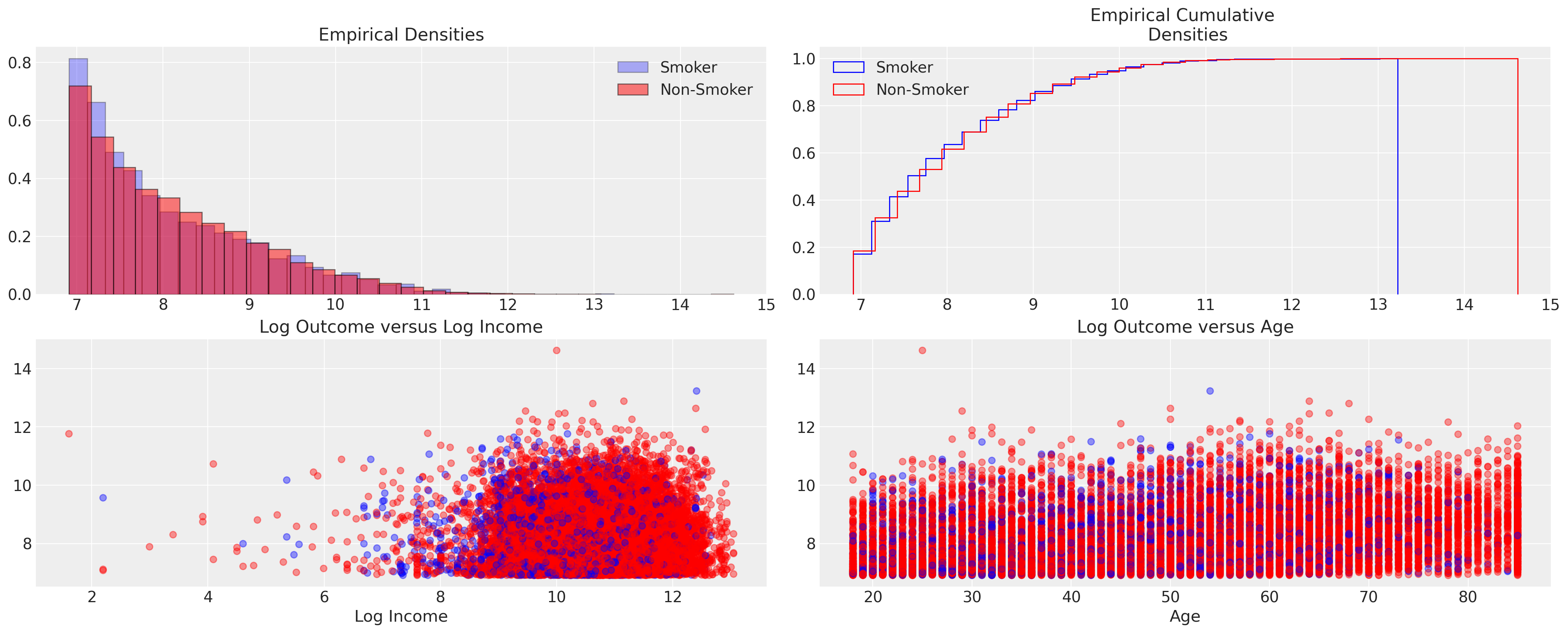
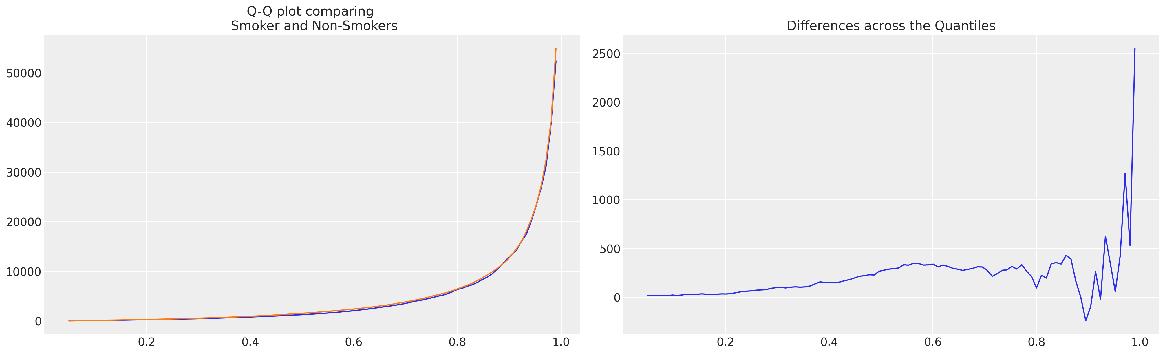
The plots would seem to confirm undifferentiated nature of the outcome across the two groups. With some hint of difference at the outer quantiles of the distribution. This is important because it suggests a minimal treatment effect on average. The outcome is recorded on the log-dollar scale, so any kind of unit movement here is quite substantial.

qs = np.linspace(0.05, 0.99, 100)
quantile_diff = (
    df.groupby("smoke")[["totexp"]]
    .quantile(qs)
    .reset_index()
    .pivot(index="level_1", columns="smoke", values="totexp")
    .rename({0: "Non-Smoker", 1: "Smoker"}, axis=1)
    .assign(diff=lambda x: x["Non-Smoker"] - x["Smoker"])
    .reset_index()
    .rename({"level_1": "quantile"}, axis=1)
)

fig, axs = plt.subplots(1, 2, figsize=(20, 6))
axs[0].plot(quantile_diff["quantile"], quantile_diff["Smoker"])
axs[0].plot(quantile_diff["quantile"], quantile_diff["Non-Smoker"])
axs[0].set_title("Q-Q plot comparing \n Smoker and Non-Smokers")
axs[1].plot(quantile_diff["quantile"], quantile_diff["diff"])
axs[1].set_title("Differences across the Quantiles");

What could go wrong?

Now we prepare the data using simple dummy encoding for the categorical variables and sample from the data set a thousand observations for our initial modelling.

dummies = pd.concat(
    [
        pd.get_dummies(df["seatbelt"], drop_first=True, prefix="seatbelt"),
        pd.get_dummies(df["marital"], drop_first=True, prefix="marital"),
        pd.get_dummies(df["race"], drop_first=True, prefix="race"),
        pd.get_dummies(df["sex"], drop_first=True, prefix="sex"),
        pd.get_dummies(df["phealth"], drop_first=True, prefix="phealth"),
    ],
    axis=1,
)
idx = df.sample(1000, random_state=100).index
X = pd.concat(
    [
        df[["age", "bmi"]],
        dummies,
    ],
    axis=1,
)
X = X.iloc[idx]
t = df.iloc[idx]["smoke"]
y = df.iloc[idx]["log_y"]
X

	age	bmi	seatbelt_Always	seatbelt_Never	seatbelt_NoCar	seatbelt_Seldom	seatbelt_Sometimes	marital_Married	marital_Separated	marital_Widowed	race_Black	race_Indig	race_Multi	race_PacificIslander	race_White	sex_Male	phealth_Fair	phealth_Good	phealth_Poor	phealth_Very Good
2852	27	23.7	0	0	0	0	0	1	0	0	0	0	0	0	1	1	0	0	0	0
13271	71	29.1	1	0	0	0	0	0	0	1	1	0	0	0	0	0	1	0	0	0
6786	19	21.3	1	0	0	0	0	0	1	0	0	0	0	0	1	0	0	0	0	1
15172	20	38.0	1	0	0	0	0	0	1	0	1	0	0	0	0	0	0	0	0	1
10967	22	28.7	1	0	0	0	0	1	0	0	0	0	0	0	1	0	0	0	0	1
...	...	...	...	...	...	...	...	...	...	...	...	...	...	...	...	...	...	...	...	...
5404	30	35.6	1	0	0	0	0	1	0	0	0	0	0	0	1	1	0	1	0	0
8665	80	22.0	1	0	0	0	0	0	0	1	0	0	0	0	0	1	0	0	0	0
3726	49	32.9	1	0	0	0	0	1	0	0	1	0	0	0	0	1	0	1	0	0
6075	49	34.2	1	0	0	0	0	1	0	0	0	0	0	1	0	0	0	0	0	1
795	53	28.2	1	0	0	0	0	1	0	0	0	0	0	0	1	1	0	0	0	0

1000 rows × 20 columns

m_ps_expend_bart, idata_expend_bart = make_propensity_model(
    X, t, bart=True, probit=False, samples=1000, m=80
)
m_ps_expend_logit, idata_expend_logit = make_propensity_model(X, t, bart=False, samples=1000)

Sampling: [mu, t_pred]
Multiprocess sampling (4 chains in 4 jobs)
PGBART: [mu]

100.00% [8000/8000 00:46<00:00 Sampling 4 chains, 0 divergences]

Sampling 4 chains for 1_000 tune and 1_000 draw iterations (4_000 + 4_000 draws total) took 46 seconds.
The rhat statistic is larger than 1.01 for some parameters. This indicates problems during sampling. See https://arxiv.org/abs/1903.08008 for details
The effective sample size per chain is smaller than 100 for some parameters.  A higher number is needed for reliable rhat and ess computation. See https://arxiv.org/abs/1903.08008 for details
Sampling: [t_pred]

100.00% [4000/4000 00:00<00:00]

Sampling: [b, t_pred]
Auto-assigning NUTS sampler...
Initializing NUTS using jitter+adapt_diag...
Multiprocess sampling (4 chains in 4 jobs)
NUTS: [b]

100.00% [8000/8000 00:18<00:00 Sampling 4 chains, 0 divergences]

Sampling 4 chains for 1_000 tune and 1_000 draw iterations (4_000 + 4_000 draws total) took 19 seconds.
Sampling: [t_pred]

100.00% [4000/4000 00:00<00:00]

az.plot_trace(idata_expend_bart, var_names=["mu", "p"]);

Show code cell source Hide code cell source

ps = idata_expend_bart["posterior"]["p"].mean(dim=("chain", "draw")).values
fig, axs = plt.subplots(2, 1, figsize=(20, 10))
axs = axs.flatten()
ax = axs[0]
ax1 = axs[1]
ax1.set_title("Overlap of Inverted Propensity Scores")
ax.hist(
    ps[t == 0],
    bins=30,
    ec="black",
    alpha=0.4,
    color="blue",
    label="Propensity Scores in Treated",
)
ax1.hist(
    ps[t == 0],
    bins=30,
    ec="black",
    alpha=0.4,
    color="blue",
    label="Propensity Scores in Treated",
)
ax.set_xlabel("Propensity Scores")
ax.set_ylabel("Count of Observed")
ax1.set_ylabel("Count of Observed")
ax.hist(
    ps[t == 1], bins=30, ec="black", alpha=0.6, color="red", label="Propensity Scores in Control"
)
ax1.hist(
    1 - ps[t == 1],
    bins=30,
    ec="black",
    alpha=0.6,
    color="red",
    label="Propensity Scores in Control",
)
ax.set_title("BART Model - Health Expenditure Data \n Propensity Scores per Group", fontsize=20)
ax.axvline(0.9, color="black", linestyle="--", label="Extreme Propensity Scores")
ax.axvline(0.1, color="black", linestyle="--")
ax1.axvline(0.9, color="black", linestyle="--", label="Extreme Propensity Scores")
ax1.axvline(0.1, color="black", linestyle="--")
ax.legend()

fig, ax2 = plt.subplots(figsize=(20, 6))
ax2.scatter(X["age"], y, color=t.map(colors), s=(1 / ps) * 20, ec="black", alpha=0.4)
ax2.set_xlabel("Age")
ax2.set_xlabel("Age")
ax2.set_ylabel("y")
ax2.set_ylabel("y")
ax2.set_title("Sized by IP Weights", fontsize=20)
red_patch = mpatches.Patch(color="red", label="Control")
blue_patch = mpatches.Patch(color="blue", label="Treated")
ax2.legend(handles=[red_patch, blue_patch]);

Note how the tails of each group in the histogram plots do not overlap well and we have some extreme propensity scores. This suggests that the propensity scores might not be well fitted to achieve good balancing properties.

Non-Parametric BART Propensity Model is Mis-specified

The flexibility of the BART model fit is poorly calibrated to recover the average treatment effect. Let’s evaluate the weighted outcome distributions under the robust inverse propensity weights estimate.

## Evaluate at the expected realisation of the propensity scores for each individual
ps = idata_expend_bart["posterior"]["p"].mean(dim=("chain", "draw")).values
make_plot(
    X,
    idata_expend_bart,
    ylims=[(-100, 340), (-60, 260), (-60, 260)],
    lower_bins=[np.arange(6, 15, 0.5), np.arange(2, 14, 0.5)],
    text_pos=(11, 80),
    method="robust",
    ps=ps,
)

This is a suspicious result. Evaluated at the expected values of the posterior propensity score distribution the robust IPW estimator of ATE suggests a substantial difference in the treatment and control groups. The re-weighted outcome in the third panel diverges across the control and treatment groups indicating a stark failure of balance. When a simple difference in the averages of the raw outcome show close to 0 differences but the re-weighted difference shows a movement of more than 1 on the log-scale. What is going on? In what follows we’ll interrogate this question from a couple of different perspectives but you should be pretty dubious of this result as it stands.

What happens if we look at the posterior ATE distributions under different estimators?

qs = range(4000)
ate_dist = [get_ate(X, t, y, q, idata_expend_bart, method="doubly_robust") for q in qs]
ate_dist_df_dr = pd.DataFrame(ate_dist, columns=["ATE", "E(Y(1))", "E(Y(0))"])

ate_dist = [get_ate(X, t, y, q, idata_expend_bart, method="robust") for q in qs]
ate_dist_df_r = pd.DataFrame(ate_dist, columns=["ATE", "E(Y(1))", "E(Y(0))"])

ate_dist_df_dr.head()

	ATE	E(Y(1))	E(Y(0))
0	-0.240666	7.852410	8.093076
1	-0.165757	7.920125	8.085882
2	-0.104837	7.971139	8.075976
3	-0.085442	7.992221	8.077663
4	-0.122315	7.955486	8.077801

Each row in this table shows an estimate of the average treatment effect and the re-weighted means of the outcome variable derived using the doubly robust esimtator with a draw from the posterior of the propensity score distribution implied by our BART model fit.

plot_ate(ate_dist_df_r, xy=(0.5, 300))

Deriving ATE estimates across draws from the posterior distribution and averaging these seems to give a more sensible figure, but still inflated beyond the minimalist differences our EDA suggested. If instead we use the doubly robust estimator we recover a more sensible figure again.

plot_ate(ate_dist_df_dr, xy=(-0.35, 200))

Recall that the doubly robust estimator is set up to effect a compromise between the propensity score weighting and (in our case) a simple OLS prediction. Where as long as one of the two models is well-specified this estimator can recover accurate unbiased treatment effects. In this case we see that the doubly robust estimator pulls away from the implications of our propensity scores and privileges the regression model.

We can also check if and how the balance breaks down with the BART based propensity scores threatening the validity of the inverse propensity score weighting.

temp = X.copy()
temp["ps"] = ps = idata_expend_bart["posterior"]["p"].mean(dim=("chain", "draw")).values
temp["ps_cut"] = pd.qcut(temp["ps"], 5)

plot_balance(temp, "bmi", t)

How does Regression Help?

We’ve just seen an example of how a mis-specfied machine learning model can wildly bias the causal estimates in a study. We’ve seen one means of fixing it, but how would things work out if we just tried simpler exploratory regression modelling? Regression automatically weights the data points by their extremity of their covariate profile and their prevalence in the sample. So in this sense adjusts for the outlier propensity scores in a way that the inverse weighting approach cannot.

model_ps_reg_expend, idata_ps_reg_expend = make_prop_reg_model(X, t, y, idata_expend_bart)

Sampling: [b, pred, sigma]
Auto-assigning NUTS sampler...
Initializing NUTS using jitter+adapt_diag...
Multiprocess sampling (4 chains in 4 jobs)
NUTS: [sigma, b]

100.00% [8000/8000 00:01<00:00 Sampling 4 chains, 0 divergences]

Sampling 4 chains for 1_000 tune and 1_000 draw iterations (4_000 + 4_000 draws total) took 1 seconds.
Sampling: [pred]

100.00% [4000/4000 00:00<00:00]

az.summary(idata_ps_reg_expend, var_names=["b"])

	mean	sd	hdi_3%	hdi_97%	mcse_mean	mcse_sd	ess_bulk	ess_tail	r_hat
b[ps]	25.533	0.774	23.977	26.884	0.016	0.011	2489.0	2640.0	1.0
b[trt]	1.393	0.386	0.670	2.118	0.008	0.005	2569.0	2348.0	1.0
b[trt*ps]	-2.079	0.964	-4.026	-0.388	0.019	0.014	2588.0	2403.0	1.0

This model is clearly too simple. It recovers only the biased estimate due to the mis-specified BART propensity model, but what if we just used the propensity as another feature in our covariate profile. Let it add precision, but fit the model we think actually reflects the causal story.

model_ps_reg_expend_h, idata_ps_reg_expend_h = make_prop_reg_model(
    X,
    t,
    y,
    idata_expend_bart,
    covariates=["age", "bmi", "phealth_Fair", "phealth_Good", "phealth_Poor", "phealth_Very Good"],
)

Sampling: [b, pred, sigma]
Auto-assigning NUTS sampler...
Initializing NUTS using jitter+adapt_diag...
Multiprocess sampling (4 chains in 4 jobs)
NUTS: [sigma, b]

100.00% [8000/8000 00:02<00:00 Sampling 4 chains, 0 divergences]

Sampling 4 chains for 1_000 tune and 1_000 draw iterations (4_000 + 4_000 draws total) took 3 seconds.
Sampling: [pred]

100.00% [4000/4000 00:00<00:00]

az.summary(idata_ps_reg_expend_h, var_names=["b"])

	mean	sd	hdi_3%	hdi_97%	mcse_mean	mcse_sd	ess_bulk	ess_tail	r_hat
b[ps]	8.799	0.588	7.759	9.963	0.010	0.007	3446.0	2897.0	1.0
b[trt]	0.098	0.245	-0.364	0.553	0.004	0.004	3737.0	3063.0	1.0
b[trt*ps]	-2.410	0.791	-3.851	-0.910	0.014	0.010	3392.0	2990.0	1.0
b[age]	0.065	0.002	0.061	0.070	0.000	0.000	3917.0	2809.0	1.0
b[bmi]	0.090	0.005	0.082	0.099	0.000	0.000	3688.0	2590.0	1.0
b[phealth_Fair]	0.285	0.180	-0.051	0.625	0.003	0.002	3234.0	2768.0	1.0
b[phealth_Good]	0.409	0.149	0.150	0.701	0.003	0.002	2882.0	2797.0	1.0
b[phealth_Poor]	0.730	0.254	0.220	1.174	0.004	0.003	3532.0	2584.0	1.0
b[phealth_Very Good]	1.328	0.132	1.084	1.579	0.002	0.002	2975.0	2947.0	1.0

This is much better and we can see that modelling the propensity score feature in conjunction with the health factors leads to a more sensible treatement effect estimate. This kind of finding echoes the lesson reported in Angrist and Pischke that:

“Regression control for the right covariates does a reasonable job of eliminating selection effects…” pg 91 Mostly Harmless Econometrics Angrist and Pischke [2008]

So we’re back to the question of the right controls. There is a no real way to avoid this burden. Machine learning cannot serve as a panacea absent domain knowledge and careful attention to the problem at hand. This is never the inspiring message people want to hear, but it is unfortunately true. Regression helps with this because the unforgiving clarity of a coefficiencts table is a reminder that there is no substitute to measuring the right things well.

Double/Debiased Machine Learning and Frisch-Waugh-Lovell

To recap - we’ve seen two examples of causal inference with inverse probability weighted adjustments. We’ve seen when it works when the propensity score model is well-calibrated. We’ve seen when it fails and how the failure can be fixed. These are tools in our tool belt - apt for different problems, but come with the requirement that we think carefully about the data generating process and the type of appropriate covariates.

In the case where the simple propensity modelling approach failed, we saw a data set in which our treatment assignment did not distinguish an average treatment effect. We also saw how if we augment our propensity based estimator we can improve the identification properties of the technique. Here we’ll show another example of how propensity models can be combined with an insight from regression based modelling to take advantage of the flexible modelling possibilities offered by machine learning approaches to causal inference. In this secrion we draw heavily on the work of Matheus Facure, especially his book Causal Inference in Python Facure [2023] but the original ideas are to be found in Victor et al. [2018]

The Frisch-Waugh-Lovell Theorem

The idea of the theorem is that for any OLS fitted linear model with a focal parameter \(\beta_{1}\) and the auxilary parameters \(\gamma_{i}\)

\[\hat{Y} = \beta_{0} + \beta_{1}D_{1} + \gamma_{1}Z_{1} + ... + \gamma_{n}Z_{n} \]

We can retrieve the same values \(\beta_{i}, \gamma_{i}\) in a two step procedure:

• Regress \(Y\) on the auxilary covariates i.e. \(\hat{Y} = \gamma_{1}Z_{1} + ... + \gamma_{n}Z_{n} \)

• Regress \(D_{1}\) on the same auxilary terms i.e. \(\hat{D_{1}} = \gamma_{1}Z_{1} + ... + \gamma_{n}Z_{n}\)

• Take the residuals \(r(D) = D_{1} - \hat{D_{1}}\) and \(r(Y) = Y - \hat{Y}\)

• Fit the regression \(r(Y) = \beta_{0} + \beta_{1}r(D)\) to find \(\beta_{1}\)

The idea of debiased machine learning is to replicate this exercise, but avail of the flexibility for machine learning models to estimate the two residual terms in the case where the focal variable of interest is our treatment variable.

This is tied to the requirement for strong ignorability because by using this process with the focal variable as \(T\) we create the treatment variable \(r(T)\) which by construction cannot be predicted from the covariate profile \(X\) ensuring \(T \perp\!\!\!\perp X\). This is a beautiful combination of ideas!

Avoiding Overfitting with K-fold Cross Validation

As we’ve seen above one of the concerns with the automatic regularisation effects of BART like tree based models is their tendency to over-fit to the seen data. Here we’ll use K-fold cross validation to generate predictions on out of sample cuts of the data. This step is crucial to avoid the over-fitting of the model to the sample data and thereby avoiding the miscalibration effects we’ve seen above. This too, (it’s easily forgotten), is a corrective step to avoid known biases due to over-indexing on the observed sample data. Using the propensity scores to achieve balance when we estimate the propensity scores on a particular sample breaks down in cases of overfit. In that case our propensity model is too aligned with the specifics of the sample and cannot serve the role of being a measure of similarity in the population.

dummies = pd.concat(
    [
        pd.get_dummies(df["seatbelt"], drop_first=True, prefix="seatbelt"),
        pd.get_dummies(df["marital"], drop_first=True, prefix="marital"),
        pd.get_dummies(df["race"], drop_first=True, prefix="race"),
        pd.get_dummies(df["sex"], drop_first=True, prefix="sex"),
        pd.get_dummies(df["phealth"], drop_first=True, prefix="phealth"),
    ],
    axis=1,
)
train_dfs = []
temp = pd.concat([df[["age", "bmi"]], dummies], axis=1)

for i in range(4):
    idx = temp.sample(1000, random_state=100).index
    X = temp.iloc[idx].copy()
    t = df.iloc[idx]["smoke"]
    y = df.iloc[idx]["log_y"]
    train_dfs.append([X, t, y])
    remaining = [True if not i in idx else False for i in temp.index]
    temp = temp[remaining]
    temp.reset_index(inplace=True, drop=True)

Applying Debiased ML Methods

Next we define the functions to fit and predict with the propensity score and outcome models. Because we’re Bayesian we will record the posterior distribution of the residuals for both the outcome model and the propensity model. In both cases we’ll use the baseline BART specification to avail of the flexibility of machine learning for accuracy. We then use the K-fold process to fit the model and predict the residuals on the out of sample fold. This allows us to extract the posterior distribution for ATE by post-processing the posterior predictive distribution of the residuals.

def train_outcome_model(X, y, m=50):
    coords = {"coeffs": list(X.columns), "obs": range(len(X))}
    with pm.Model(coords=coords) as model:
        X_data = pm.MutableData("X", X)
        y_data = pm.MutableData("y_data", y)
        mu = pmb.BART("mu", X_data, y, m=m)
        sigma = pm.HalfNormal("sigma", 1)
        obs = pm.Normal("obs", mu, sigma, observed=y_data)
        idata = pm.sample_prior_predictive()
        idata.extend(pm.sample(1000, progressbar=False))
    return model, idata


def train_propensity_model(X, t, m=50):
    coords = {"coeffs": list(X.columns), "obs_id": range(len(X))}
    with pm.Model(coords=coords) as model_ps:
        X_data = pm.MutableData("X", X)
        t_data = pm.MutableData("t_data", t)
        mu = pmb.BART("mu", X_data, t, m=m)
        p = pm.Deterministic("p", pm.math.invlogit(mu))
        t_pred = pm.Bernoulli("obs", p=p, observed=t_data)
        idata = pm.sample_prior_predictive()
        idata.extend(pm.sample(1000, progressbar=False))
    return model_ps, idata


def cross_validate(train_dfs, test_idx):
    test = train_dfs[test_idx]
    test_X = test[0]
    test_t = test[1]
    test_y = test[2]
    train_X = pd.concat([train_dfs[i][0] for i in range(4) if i != test_idx])
    train_t = pd.concat([train_dfs[i][1] for i in range(4) if i != test_idx])
    train_y = pd.concat([train_dfs[i][2] for i in range(4) if i != test_idx])

    model, idata = train_outcome_model(train_X, train_y)
    with model:
        pm.set_data({"X": test_X, "y_data": test_y})
        idata_pred = pm.sample_posterior_predictive(idata)
    y_resid = idata_pred["posterior_predictive"]["obs"].stack(z=("chain", "draw")).T - test_y.values

    model_t, idata_t = train_propensity_model(train_X, train_t)
    with model_t:
        pm.set_data({"X": test_X, "t_data": test_t})
        idata_pred_t = pm.sample_posterior_predictive(idata_t)
    t_resid = (
        idata_pred_t["posterior_predictive"]["obs"].stack(z=("chain", "draw")).T - test_t.values
    )

    return y_resid, t_resid, idata_pred, idata_pred_t


y_resids = []
t_resids = []
model_fits = {}
for i in range(4):
    y_resid, t_resid, idata_pred, idata_pred_t = cross_validate(train_dfs, i)
    y_resids.append(y_resid)
    t_resids.append(t_resid)
    t_effects = []
    for j in range(1000):
        intercept = np.ones_like(1000)
        covariates = pd.DataFrame({"intercept": intercept, "t_resid": t_resid[j, :].values})
        m0 = sm.OLS(y_resid[j, :].values, covariates).fit()
        t_effects.append(m0.params["t_resid"])
    model_fits[i] = [m0, t_effects]
    print(f"Estimated Treament Effect in K-fold {i}: {np.mean(t_effects)}")

Show code cell output Hide code cell output

Sampling: [mu, obs, sigma]
Multiprocess sampling (4 chains in 4 jobs)
CompoundStep
>PGBART: [mu]
>NUTS: [sigma]
Sampling 4 chains for 1_000 tune and 1_000 draw iterations (4_000 + 4_000 draws total) took 31 seconds.
The rhat statistic is larger than 1.01 for some parameters. This indicates problems during sampling. See https://arxiv.org/abs/1903.08008 for details
The effective sample size per chain is smaller than 100 for some parameters.  A higher number is needed for reliable rhat and ess computation. See https://arxiv.org/abs/1903.08008 for details
Sampling: [mu, obs]

100.00% [4000/4000 00:16<00:00]

Sampling: [mu, obs]
Multiprocess sampling (4 chains in 4 jobs)
PGBART: [mu]
Sampling 4 chains for 1_000 tune and 1_000 draw iterations (4_000 + 4_000 draws total) took 51 seconds.
The rhat statistic is larger than 1.01 for some parameters. This indicates problems during sampling. See https://arxiv.org/abs/1903.08008 for details
The effective sample size per chain is smaller than 100 for some parameters.  A higher number is needed for reliable rhat and ess computation. See https://arxiv.org/abs/1903.08008 for details
Sampling: [mu, obs]

100.00% [4000/4000 00:14<00:00]

Estimated Treament Effect in K-fold 0: -0.007055724114450991

Sampling: [mu, obs, sigma]
Multiprocess sampling (4 chains in 4 jobs)
CompoundStep
>PGBART: [mu]
>NUTS: [sigma]
Sampling 4 chains for 1_000 tune and 1_000 draw iterations (4_000 + 4_000 draws total) took 31 seconds.
The rhat statistic is larger than 1.01 for some parameters. This indicates problems during sampling. See https://arxiv.org/abs/1903.08008 for details
The effective sample size per chain is smaller than 100 for some parameters.  A higher number is needed for reliable rhat and ess computation. See https://arxiv.org/abs/1903.08008 for details
Sampling: [mu, obs]

100.00% [4000/4000 00:16<00:00]

Sampling: [mu, obs]
Multiprocess sampling (4 chains in 4 jobs)
PGBART: [mu]
Sampling 4 chains for 1_000 tune and 1_000 draw iterations (4_000 + 4_000 draws total) took 50 seconds.
The rhat statistic is larger than 1.01 for some parameters. This indicates problems during sampling. See https://arxiv.org/abs/1903.08008 for details
The effective sample size per chain is smaller than 100 for some parameters.  A higher number is needed for reliable rhat and ess computation. See https://arxiv.org/abs/1903.08008 for details
Sampling: [mu, obs]

100.00% [4000/4000 00:15<00:00]

Estimated Treament Effect in K-fold 1: -0.0381788005862483

Sampling: [mu, obs, sigma]
Multiprocess sampling (4 chains in 4 jobs)
CompoundStep
>PGBART: [mu]
>NUTS: [sigma]
Sampling 4 chains for 1_000 tune and 1_000 draw iterations (4_000 + 4_000 draws total) took 31 seconds.
The rhat statistic is larger than 1.01 for some parameters. This indicates problems during sampling. See https://arxiv.org/abs/1903.08008 for details
The effective sample size per chain is smaller than 100 for some parameters.  A higher number is needed for reliable rhat and ess computation. See https://arxiv.org/abs/1903.08008 for details
Sampling: [mu, obs]

100.00% [4000/4000 00:15<00:00]

Sampling: [mu, obs]
Multiprocess sampling (4 chains in 4 jobs)
PGBART: [mu]
Sampling 4 chains for 1_000 tune and 1_000 draw iterations (4_000 + 4_000 draws total) took 50 seconds.
The rhat statistic is larger than 1.01 for some parameters. This indicates problems during sampling. See https://arxiv.org/abs/1903.08008 for details
The effective sample size per chain is smaller than 100 for some parameters.  A higher number is needed for reliable rhat and ess computation. See https://arxiv.org/abs/1903.08008 for details
Sampling: [mu, obs]

100.00% [4000/4000 00:15<00:00]

Estimated Treament Effect in K-fold 2: -0.03088459747780483

Sampling: [mu, obs, sigma]
Multiprocess sampling (4 chains in 4 jobs)
CompoundStep
>PGBART: [mu]
>NUTS: [sigma]
Sampling 4 chains for 1_000 tune and 1_000 draw iterations (4_000 + 4_000 draws total) took 31 seconds.
The rhat statistic is larger than 1.01 for some parameters. This indicates problems during sampling. See https://arxiv.org/abs/1903.08008 for details
The effective sample size per chain is smaller than 100 for some parameters.  A higher number is needed for reliable rhat and ess computation. See https://arxiv.org/abs/1903.08008 for details
Sampling: [mu, obs]

100.00% [4000/4000 00:16<00:00]

Sampling: [mu, obs]
Multiprocess sampling (4 chains in 4 jobs)
PGBART: [mu]
Sampling 4 chains for 1_000 tune and 1_000 draw iterations (4_000 + 4_000 draws total) took 51 seconds.
The rhat statistic is larger than 1.01 for some parameters. This indicates problems during sampling. See https://arxiv.org/abs/1903.08008 for details
The effective sample size per chain is smaller than 100 for some parameters.  A higher number is needed for reliable rhat and ess computation. See https://arxiv.org/abs/1903.08008 for details
Sampling: [mu, obs]

100.00% [4000/4000 00:15<00:00]

Estimated Treament Effect in K-fold 3: 0.0012725964211934963

y_resids_stacked = xr.concat(y_resids, dim=("obs_dim_2"))
t_resids_stacked = xr.concat(t_resids, dim=("obs_dim_2"))

y_resids_stacked

<xarray.DataArray 'obs' (z: 4000, obs_dim_2: 4000)>
array([[ 2.12096806, -0.18759006,  1.65643341, ...,  0.96914617,
        -1.09227918,  0.79439211],
       [-0.2475453 , -1.71716078,  0.90773827, ...,  1.9150216 ,
         0.22575749,  1.205472  ],
       [ 1.84052802, -0.06495813,  1.13329414, ...,  0.33619207,
        -0.97017944,  1.55807636],
       ...,
       [ 1.11205571,  0.00451481, -0.11181589, ...,  3.16765911,
        -1.85359818,  1.12836815],
       [ 0.60629988,  0.96163265,  1.32810649, ...,  1.97479916,
        -0.09903109,  1.37666937],
       [ 0.52163258, -0.11855604, -0.28945473, ...,  0.24204002,
        -0.6780746 ,  0.18923211]])
Coordinates:
  * obs_dim_2  (obs_dim_2) int64 0 1 2 3 4 5 6 7 ... 993 994 995 996 997 998 999
  * z          (z) object MultiIndex
  * chain      (z) int64 0 0 0 0 0 0 0 0 0 0 0 0 0 ... 3 3 3 3 3 3 3 3 3 3 3 3 3
  * draw       (z) int64 0 1 2 3 4 5 6 7 8 ... 992 993 994 995 996 997 998 999

xarray.DataArray

'obs'

• z: 4000
• obs_dim_2: 4000

• 2.121 -0.1876 1.656 -0.4564 0.6595 ... 1.499 0.242 -0.6781 0.1892

  array([[ 2.12096806, -0.18759006,  1.65643341, ...,  0.96914617,
          -1.09227918,  0.79439211],
         [-0.2475453 , -1.71716078,  0.90773827, ...,  1.9150216 ,
           0.22575749,  1.205472  ],
         [ 1.84052802, -0.06495813,  1.13329414, ...,  0.33619207,
          -0.97017944,  1.55807636],
         ...,
         [ 1.11205571,  0.00451481, -0.11181589, ...,  3.16765911,
          -1.85359818,  1.12836815],
         [ 0.60629988,  0.96163265,  1.32810649, ...,  1.97479916,
          -0.09903109,  1.37666937],
         [ 0.52163258, -0.11855604, -0.28945473, ...,  0.24204002,
          -0.6780746 ,  0.18923211]])

• Coordinates: (4)
  • obs_dim_2
    (obs_dim_2)
    int64
    0 1 2 3 4 5 ... 995 996 997 998 999

    array([  0,   1,   2, ..., 997, 998, 999])

  • z
    (z)
    object
    MultiIndex

    array([(0, 0), (0, 1), (0, 2), ..., (3, 997), (3, 998), (3, 999)], dtype=object)

  • chain
    (z)
    int64
    0 0 0 0 0 0 0 0 ... 3 3 3 3 3 3 3 3

    array([0, 0, 0, ..., 3, 3, 3])

  • draw
    (z)
    int64
    0 1 2 3 4 5 ... 995 996 997 998 999

    array([  0,   1,   2, ..., 997, 998, 999])

• Indexes: (2)
  • obs_dim_2
    PandasIndex

    PandasIndex(Int64Index([  0,   1,   2,   3,   4,   5,   6,   7,   8,   9,
                ...
                990, 991, 992, 993, 994, 995, 996, 997, 998, 999],
               dtype='int64', name='obs_dim_2', length=4000))

  • z
    chain
    draw
    PandasMultiIndex

    PandasIndex(MultiIndex([(0,   0),
                (0,   1),
                (0,   2),
                (0,   3),
                (0,   4),
                (0,   5),
                (0,   6),
                (0,   7),
                (0,   8),
                (0,   9),
                ...
                (3, 990),
                (3, 991),
                (3, 992),
                (3, 993),
                (3, 994),
                (3, 995),
                (3, 996),
                (3, 997),
                (3, 998),
                (3, 999)],
               name='z', length=4000))

• Attributes: (0)

Post process the posterior predictive distribution of residuals

t_effects = []
intercepts = []
for i in range(4000):
    intercept = np.ones_like(4000)
    covariates = pd.DataFrame({"intercept": intercept, "t_resid": t_resids_stacked[i, :].values})
    m0 = sm.OLS(y_resids_stacked[i, :].values, covariates).fit()
    t_effects.append(m0.params["t_resid"])
    intercepts.append(m0.params["intercept"])

fig, axs = plt.subplots(1, 2, figsize=(15, 6))
axs = axs.flatten()
axs[0].hist(t_effects, bins=30, ec="black", color="slateblue", label="ATE", density=True, alpha=0.6)
x = np.linspace(-1, 1, 10)
for i in range(1000):
    axs[1].plot(x, intercepts[i] + t_effects[i] * x, color="darkred", alpha=0.3)

axs[0].set_title("Double ML - ATE estimate \n Distribution")
axs[1].set_title(r" Posterior Regression Line of Residuals: r(Y) ~ $\beta$r(T)")
ate = np.mean(t_effects)
axs[0].axvline(ate, color="black", linestyle="--", label=f"E(ATE) = {np.round(ate, 2)}")
axs[1].plot(x, np.mean(intercepts) + np.mean(t_effects) * x, color="black", label="Expected Fit")
axs[1].legend()
axs[0].legend();

We can see here how the technique of debiased machine learning has helped to alleviate some of the miscalibrated effects of naively fitting the BART model to the propensity score estimation task. Additionally we now have quantified some of the uncertainty in the ATE which determines a relatively flat regression line on the residuals.

Conditional Average Treatment Effects

We’ll note here that Double ML approaches also offer another lens on the problem. They allow you to move away from the focus on Average Treatment Effects and retrieve estimates more tailored to the individual covariate profiles. Much of the theoretical detail is elaborated in Facure [2023] and we won’t cover it here apart from suggesting that it makes good sense to use the residual prediction in estimating specific treatment effects. We’ll show here briefly how to build on the derived residuals to retrieve the CATE estimates using the flexibility of machine learning to better capture the range of heterogenous treatment effects.

def make_cate(y_resids_stacked, t_resids_stacked, train_dfs, i, method="forest"):
    train_X = pd.concat([train_dfs[i][0] for i in range(4)])
    train_t = pd.concat([train_dfs[i][1] for i in range(4)])

    df_cate = pd.DataFrame(
        {"y_r": y_resids_stacked[i, :].values, "t_r": t_resids_stacked[i, :].values}
    )
    df_cate["target"] = df_cate["y_r"] / np.where(
        df_cate["t_r"] == 0, df_cate["t_r"] + 1e-25, df_cate["t_r"]
    )
    df_cate["weight"] = df_cate["t_r"] ** 2
    train_X.reset_index(drop=True, inplace=True)
    train_t.reset_index(drop=True, inplace=True)
    if method == "forest":
        CATE_model = RandomForestRegressor()
        CATE_model.fit(train_X, df_cate["target"], sample_weight=df_cate["weight"])
    elif method == "gradient":
        CATE_model = GradientBoostingRegressor()
        CATE_model.fit(train_X, df_cate["target"], sample_weight=df_cate["weight"])
    else:
        CATE_model = sm.WLS(df_cate["target"], train_X, weights=df_cate["weight"])
        CATE_model = CATE_model.fit()
    df_cate["CATE"] = CATE_model.predict(train_X)
    df_cate["t"] = train_t
    return df_cate

Show code cell source Hide code cell source

fig, axs = plt.subplots(1, 3, figsize=(20, 7))
axs = axs.flatten()

q_95 = []
for i in range(100):
    cate_df = make_cate(y_resids_stacked, t_resids_stacked, train_dfs, i)
    axs[1].hist(
        cate_df[cate_df["t"] == 0]["CATE"],
        bins=30,
        alpha=0.1,
        color="red",
        density=True,
    )
    q_95.append(
        [
            cate_df[cate_df["t"] == 0]["CATE"].quantile(0.99),
            cate_df[cate_df["t"] == 1]["CATE"].quantile(0.99),
            cate_df[cate_df["t"] == 0]["CATE"].quantile(0.01),
            cate_df[cate_df["t"] == 1]["CATE"].quantile(0.01),
        ]
    )
    axs[1].hist(cate_df[cate_df["t"] == 1]["CATE"], bins=30, alpha=0.1, color="blue", density=True)
axs[1].set_title(
    "CATE Predictions \n Estimated across Posterior of Residuals", fontsize=20, fontweight="bold"
)

q_df = pd.DataFrame(q_95, columns=["Control_p99", "Treated_p99", "Control_p01", "Treated_p01"])
axs[2].hist(q_df["Treated_p99"], ec="black", color="blue", alpha=0.4, label="Treated p99")
axs[2].hist(q_df["Control_p99"], ec="black", color="red", alpha=0.4, label="Control p99")
axs[2].legend()
axs[2].set_title("Distribution of p99 CATE predictions")
axs[0].hist(q_df["Treated_p01"], ec="black", color="blue", alpha=0.4, label="Treated p01")
axs[0].hist(q_df["Control_p01"], ec="black", color="red", alpha=0.4, label="Control p01")
axs[0].legend()
axs[0].set_title("Distribution of p01 CATE predictions");

This perspective starts to show the importance of heterogeneity in causal impacts and offers a means of assessing differential impact of treatments. However, while the treated population (i.e. the smokers’s) are implied to have longer tails and more extreme outcomes - you might wonder why the effect is somewhat symmetrical? Why would they also exhibit less extreme expenditures too?

Mediation Effects and Causal Structure

Above we’ve seen how a number of different approaches designed to avoid bias lead us to the conclusion that smoking has limited or no effect on your likely healthcare costs. It’s worth emphasising that this should strike you as strange!

The solution to the puzzle lies not in the method of estimation precisely, but in the structure of the question. It’s not that smoking isn’t related to healthcare costs, but that the impact is mediated through smoking’s influence on our health.

The structural imposition of mediation mandates valid causal inferences go through just when sequential ignorability holds. That is to say - the potential outcomes are independent of the treatment assignment history conditional on covariate profiles. More detail can be found in Daniels et al. [2024]. But we can see how this works if we write the mediation structure into our model as described in Bayesian mediation analysis. The fundamental point is that we need to augment our modelling to account for the structure of the causal flow. This is a substantive structural belief about the data generating process which we impose in the model of the joint distribution for mediator and outcome.

fig, ax = plt.subplots(figsize=(20, 6))
graph = nx.DiGraph()
graph.add_node("T")
graph.add_node("M")
graph.add_node("Y")
graph.add_edges_from([("T", "M"), ("M", "Y"), ("T", "Y")])

nx.draw(
    graph,
    arrows=True,
    with_labels=True,
    pos={"T": (1, 2), "M": (1.8, 3), "Y": (3, 1)},
    ax=ax,
    node_size=6000,
    font_color="whitesmoke",
    font_size=20,
)

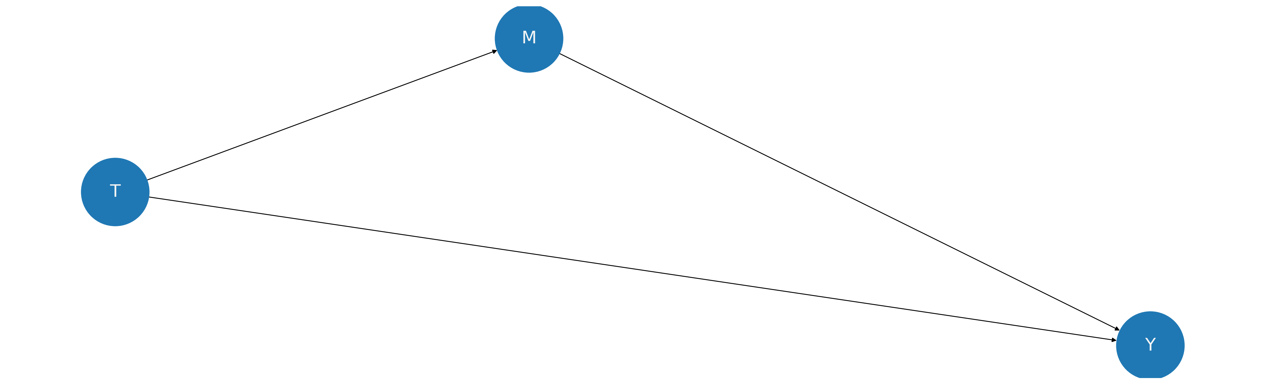
Here the treatment T flows through the mediator M to impact the outcome Y while simultaneously directly impacting the outcome.

dummies = pd.concat(
    [
        pd.get_dummies(df["seatbelt"], drop_first=True, prefix="seatbelt"),
        pd.get_dummies(df["marital"], drop_first=True, prefix="marital"),
        pd.get_dummies(df["race"], drop_first=True, prefix="race"),
        pd.get_dummies(df["sex"], drop_first=True, prefix="sex"),
        pd.get_dummies(df["phealth"], drop_first=True, prefix="phealth"),
    ],
    axis=1,
)
idx = df.sample(5000, random_state=100).index
X = pd.concat(
    [
        df[["age", "bmi"]],
        dummies,
    ],
    axis=1,
)
X = X.iloc[idx]
t = df.iloc[idx]["smoke"]
y = df.iloc[idx]["log_y"]
X


lkup = {
    "phealth_Poor": 1,
    "phealth_Fair": 2,
    "phealth_Good": 3,
    "phealth_Very Good": 4,
    "phealth_Excellent": 5,
}

### Construct the health status variables as an ordinal rank
### to use the health rank as a mediator for smoking.
m = pd.DataFrame(
    (
        pd.from_dummies(
            X[["phealth_Poor", "phealth_Fair", "phealth_Good", "phealth_Very Good"]],
            default_category="phealth_Excellent",
        ).values.flatten()
    ),
    columns=["health"],
)["health"].map(lkup)

X_m = X.copy().drop(["phealth_Poor", "phealth_Fair", "phealth_Good", "phealth_Very Good"], axis=1)
X_m

	age	bmi	seatbelt_Always	seatbelt_Never	seatbelt_NoCar	seatbelt_Seldom	seatbelt_Sometimes	marital_Married	marital_Separated	marital_Widowed	race_Black	race_Indig	race_Multi	race_PacificIslander	race_White	sex_Male
2852	27	23.7	0	0	0	0	0	1	0	0	0	0	0	0	1	1
13271	71	29.1	1	0	0	0	0	0	0	1	1	0	0	0	0	0
6786	19	21.3	1	0	0	0	0	0	1	0	0	0	0	0	1	0
15172	20	38.0	1	0	0	0	0	0	1	0	1	0	0	0	0	0
10967	22	28.7	1	0	0	0	0	1	0	0	0	0	0	0	1	0
...	...	...	...	...	...	...	...	...	...	...	...	...	...	...	...	...
1135	51	29.8	0	0	0	0	0	0	1	0	0	0	0	0	1	0
1706	50	26.6	1	0	0	0	0	1	0	0	0	0	0	0	1	0
11205	24	23.7	1	0	0	0	0	0	1	0	0	0	0	0	1	0
12323	36	35.9	1	0	0	0	0	0	0	0	1	0	0	0	0	1
15604	29	-9.0	1	0	0	0	0	0	1	0	0	0	0	0	1	0

5000 rows × 16 columns

We define a flexible model which estimates the outcome using a BART model and estimates the mediating variable using a simpler linear regression. However we embed both in a linear equation to capture the coefficients required to “read-off” the total, indirect and direct effects of smoking on health expenditure as mediated by health.

def mediation_model(X_m, t, m, y):
    with pm.Model(coords={"coeffs": list(X_m.columns), "obs_id": range(len(X_m))}) as model:
        t_data = pm.MutableData("t", t, dims="obs_id")
        m = pm.MutableData("m", m, dims="obs_id")
        X_data = pm.MutableData("X", X_m)

        # intercept priors
        im = pm.Normal("im", mu=0, sigma=10)
        iy = pm.Normal("iy", mu=0, sigma=10)
        # slope priors
        a = pm.Normal("a", mu=0, sigma=1)
        b = pm.Normal("b", mu=0, sigma=1)
        cprime = pm.Normal("cprime", mu=0, sigma=1)
        # noise priors
        sigma1 = pm.Exponential("sigma1", 1)
        sigma2 = pm.Exponential("sigma2", 1)
        bart_mu = pmb.BART("mu", X_data, y)
        beta = pm.Normal("beta", mu=0, sigma=1, dims="coeffs")
        mu_m = pm.Deterministic("mu_m", pm.math.dot(X_data, beta), dims="obs_id")

        # likelihood
        pm.Normal(
            "mlikelihood", mu=(im + a * t_data) + mu_m, sigma=sigma1, observed=m, dims="obs_id"
        )
        pm.Normal(
            "ylikelihood",
            mu=iy + b * m + cprime * t_data + bart_mu,
            sigma=sigma2,
            observed=y,
            dims="obs_id",
        )

        # calculate quantities of interest
        indirect_effect = pm.Deterministic("indirect effect", a * b)
        total_effect = pm.Deterministic("total effect", a * b + cprime)

    return model


model = mediation_model(X_m, t, m, y)
pm.model_to_graphviz(model)

with model:
    result = pm.sample(tune=1000, random_seed=42, target_accept=0.95)

Multiprocess sampling (4 chains in 4 jobs)
CompoundStep
>NUTS: [im, iy, a, b, cprime, sigma1, sigma2, beta]
>PGBART: [mu]

100.00% [8000/8000 02:44<00:00 Sampling 4 chains, 0 divergences]

Sampling 4 chains for 1_000 tune and 1_000 draw iterations (4_000 + 4_000 draws total) took 164 seconds.
The rhat statistic is larger than 1.01 for some parameters. This indicates problems during sampling. See https://arxiv.org/abs/1903.08008 for details
The effective sample size per chain is smaller than 100 for some parameters.  A higher number is needed for reliable rhat and ess computation. See https://arxiv.org/abs/1903.08008 for details

ax = az.plot_posterior(
    result,
    var_names=["cprime", "indirect effect", "total effect"],
    ref_val=0,
    hdi_prob=0.95,
    figsize=(20, 6),
)
ax[0].set(title="direct effect");

Here we begin to see what’s going on. The influence of smoking is directly negative, but the indirect effect through the mediator of health status is positive and the combined effect cancels out/reduces the treatment effect on the outcome. Using this new structure we can of course use the regression imputation approach to causal inference and derive a kind of ceteris paribus law about the impact of smoking as mediated through the observed health features. More neatly we can derive the causal mediation estimands using the potential outcomes framework in a way that does not rely on the functional form of the outcome and mediation models.

Mediation Estimands

In mediation analysis we are committed to the view that the correct causal structure of the problem is represented by an interrupted path of influence between the treatment variable and the outcome of interest. This implies that there are expected effects of treatment but that we need to do some more work to disentangle the natural direct effect (NDE) and natural indirect effects (NIE) of treatment on outcome.

These quantities are represented using the potential outcomes notation as follows:

• Let \(M(t)\) be the value of mediator under the treatment specification \(t\).

• Then \(Y(t, M(t))\) is a “nested” potential outcome for our outcome variable Y dependent on realisation of \(M\) based on \(t\).

• Distinguish \(t\) as a specific setting for the treatment variable in \(\{ 0, 1\}\) from \(t^{*}\) as an alternative setting.

Now we define

• NDE: \(E[Y(t, M(t^{*})) - Y(t^{*}, M(t^{*}))]\)

  • Which is to say we’re interested in the differences in the outcomes under different treatments, mediated by values for M under a specific treatment regime.

• NIE: \(E[(Y(t, M(t))) - Y(t, M(t^{*}))]\)

  • Which amounts to the differences in the outcome Y due to differences in the treatment regimes which generated the mediation values M.

• TE: NDE + NIE

These equations are subtle, and the potential outcomes notation is perhaps a little obscure, but it’s the notation we inherit. The key point is just that in NDE the treatment regime for the mediation effects are fixed and the values for the outcome varied. In the NIE the values for the mediation effects are varied and the treatment regime for the outcome variable is fixed.

We are going to demonstrate how to recover the causal mediation estimands using the counterfactual imputation approach for the mediation values and substituting these imputed mediation values as appropriate into the formulas for the NDE and NIE. We base these calculations on the inference data object result derived above when we fitted the initial mediation model.

def counterfactual_mediation(model, result, X, treatment_status=1):
    if treatment_status == 1:
        t_mod = np.ones(len(X), dtype="int32")
    else:
        t_mod = np.zeros(len(X), dtype="int32")
    with model:
        # update values of predictors:
        pm.set_data({"t": t_mod})
        idata = pm.sample_posterior_predictive(result, var_names=["mlikelihood"], progressbar=False)
    return idata


### Impute Mediation values under different treatment regimes
### To be used to vary the imputation efforts of the outcome variable in the
### NDE and NIE calculations below.
idata_1m = counterfactual_mediation(model, result, X_m, treatment_status=1)
idata_0m = counterfactual_mediation(model, result, X_m, treatment_status=0)


def counterfactual_outcome(
    model, result, m_idata, sample_index=0, treatment_status=1, modified_m=True
):
    """Ensure we can change sample_index so we can post-process the mediator posterior predictive
    distributions and derive posterior predictive views of the conditional variation in the outcome.
    """
    if treatment_status == 1:
        t_mod = np.ones(len(X), dtype="int32")
        m_mod = az.extract(m_idata["posterior_predictive"]["mlikelihood"])["mlikelihood"][
            :, sample_index
        ].values.astype(int)
    else:
        t_mod = np.zeros(len(X), dtype="int32")
        m_mod = az.extract(m_idata["posterior_predictive"]["mlikelihood"])["mlikelihood"][
            :, sample_index
        ].values.astype(int)
    if not modified_m:
        m_mod = result["constant_data"]["m"].values
    with model:
        # update values of predictors:
        pm.set_data({"t": t_mod, "m": m_mod})
        idata = pm.sample_posterior_predictive(result, var_names=["ylikelihood"], progressbar=False)
    return idata


### Using one draw from the posterior of the mediation inference objects.
### We vary the treatment of the outcome but keep the Mediator values static under
### the counterfactual regime of no treatment
idata_nde1 = counterfactual_outcome(model, result, m_idata=idata_0m, treatment_status=1)
idata_nde0 = counterfactual_outcome(model, result, m_idata=idata_0m, treatment_status=0)

### We fix the treatment regime for the outcome but vary the mediator status
### between those counterfactual predictions and the observed mediator values
idata_nie0 = counterfactual_outcome(model, result, m_idata=idata_0m, treatment_status=0)
idata_nie1 = counterfactual_outcome(
    model, result, m_idata=idata_0m, treatment_status=0, modified_m=False
)

Sampling: [mlikelihood]
Sampling: [mlikelihood]
Sampling: [ylikelihood]
Sampling: [ylikelihood]
Sampling: [ylikelihood]
Sampling: [ylikelihood]

### Natural Direct Effect
nde = (
    idata_nde1["posterior_predictive"]["ylikelihood"].mean()
    - idata_nde0["posterior_predictive"]["ylikelihood"].mean()
)
nde

<xarray.DataArray 'ylikelihood' ()>
array(-0.08185824)

xarray.DataArray

'ylikelihood'

• -0.08186

  array(-0.08185824)

• Coordinates: (0)
• Indexes: (0)
• Attributes: (0)

### Natural InDirect Effect
nie = (
    idata_nie0["posterior_predictive"]["ylikelihood"].mean()
    - idata_nie1["posterior_predictive"]["ylikelihood"].mean()
)
nie

<xarray.DataArray 'ylikelihood' ()>
array(0.08437854)

xarray.DataArray

'ylikelihood'

• 0.08438

  array(0.08437854)

• Coordinates: (0)
• Indexes: (0)
• Attributes: (0)

### Total Effect
nde + nie

<xarray.DataArray 'ylikelihood' ()>
array(0.0025203)

xarray.DataArray

'ylikelihood'

• 0.00252

  array(0.0025203)

• Coordinates: (0)
• Indexes: (0)
• Attributes: (0)

Note how we recover estimates in this fashion that mirror the canonical formulas derived from the mediation model above. However, what is important is that this imputation approach is feasible regardless of the parametric construction of our mediation and outcome models.

Next we loop through draws from the counterfactual posteriors over the mediation values to derive posterior predictive distributions for the causal estimands.

estimands = []
for i in range(400):
    idata_nde1 = counterfactual_outcome(
        model, result, m_idata=idata_0m, treatment_status=1, sample_index=i
    )
    idata_nde0 = counterfactual_outcome(
        model, result, m_idata=idata_0m, treatment_status=0, sample_index=i
    )

    idata_nie0 = counterfactual_outcome(
        model, result, m_idata=idata_0m, treatment_status=0, sample_index=i
    )
    idata_nie1 = counterfactual_outcome(
        model, result, m_idata=idata_0m, treatment_status=0, modified_m=False, sample_index=i
    )

    nde = (
        idata_nde1["posterior_predictive"]["ylikelihood"].mean()
        - idata_nde0["posterior_predictive"]["ylikelihood"].mean()
    )
    nie = (
        idata_nie0["posterior_predictive"]["ylikelihood"].mean()
        - idata_nie1["posterior_predictive"]["ylikelihood"].mean()
    )
    te = nde + nie
    estimands.append([nde.item(), nie.item(), te.item()])

estimands_df = pd.DataFrame(
    estimands, columns=["Natural Direct Effect", "Natural Indirect Effect", "Total Effect"]
)

Show code cell output Hide code cell output

Sampling: [ylikelihood]
Sampling: [ylikelihood]
Sampling: [ylikelihood]
Sampling: [ylikelihood]
Sampling: [ylikelihood]
Sampling: [ylikelihood]
Sampling: [ylikelihood]
Sampling: [ylikelihood]
Sampling: [ylikelihood]
Sampling: [ylikelihood]
Sampling: [ylikelihood]
Sampling: [ylikelihood]
Sampling: [ylikelihood]
Sampling: [ylikelihood]
Sampling: [ylikelihood]
Sampling: [ylikelihood]
Sampling: [ylikelihood]
Sampling: [ylikelihood]
Sampling: [ylikelihood]
Sampling: [ylikelihood]
Sampling: [ylikelihood]
Sampling: [ylikelihood]
Sampling: [ylikelihood]
Sampling: [ylikelihood]
Sampling: [ylikelihood]
Sampling: [ylikelihood]
Sampling: [ylikelihood]
Sampling: [ylikelihood]
Sampling: [ylikelihood]
Sampling: [ylikelihood]
Sampling: [ylikelihood]
Sampling: [ylikelihood]
Sampling: [ylikelihood]
Sampling: [ylikelihood]
Sampling: [ylikelihood]
Sampling: [ylikelihood]
Sampling: [ylikelihood]
Sampling: [ylikelihood]
Sampling: [ylikelihood]
Sampling: [ylikelihood]
Sampling: [ylikelihood]
Sampling: [ylikelihood]
Sampling: [ylikelihood]
Sampling: [ylikelihood]
Sampling: [ylikelihood]
Sampling: [ylikelihood]
Sampling: [ylikelihood]
Sampling: [ylikelihood]
Sampling: [ylikelihood]
Sampling: [ylikelihood]
Sampling: [ylikelihood]
Sampling: [ylikelihood]
Sampling: [ylikelihood]
Sampling: [ylikelihood]
Sampling: [ylikelihood]
Sampling: [ylikelihood]
Sampling: [ylikelihood]
Sampling: [ylikelihood]
Sampling: [ylikelihood]
Sampling: [ylikelihood]
Sampling: [ylikelihood]
Sampling: [ylikelihood]
Sampling: [ylikelihood]
Sampling: [ylikelihood]
Sampling: [ylikelihood]
Sampling: [ylikelihood]
Sampling: [ylikelihood]
Sampling: [ylikelihood]
Sampling: [ylikelihood]
Sampling: [ylikelihood]
Sampling: [ylikelihood]
Sampling: [ylikelihood]
Sampling: [ylikelihood]
Sampling: [ylikelihood]
Sampling: [ylikelihood]
Sampling: [ylikelihood]
Sampling: [ylikelihood]
Sampling: [ylikelihood]
Sampling: [ylikelihood]
Sampling: [ylikelihood]
Sampling: [ylikelihood]
Sampling: [ylikelihood]
Sampling: [ylikelihood]
Sampling: [ylikelihood]
Sampling: [ylikelihood]
Sampling: [ylikelihood]
Sampling: [ylikelihood]
Sampling: [ylikelihood]
Sampling: [ylikelihood]
Sampling: [ylikelihood]
Sampling: [ylikelihood]
Sampling: [ylikelihood]
Sampling: [ylikelihood]
Sampling: [ylikelihood]
Sampling: [ylikelihood]
Sampling: [ylikelihood]
Sampling: [ylikelihood]
Sampling: [ylikelihood]
Sampling: [ylikelihood]
Sampling: [ylikelihood]
Sampling: [ylikelihood]
Sampling: [ylikelihood]
Sampling: [ylikelihood]
Sampling: [ylikelihood]
Sampling: [ylikelihood]
Sampling: [ylikelihood]
Sampling: [ylikelihood]
Sampling: [ylikelihood]
Sampling: [ylikelihood]
Sampling: [ylikelihood]
Sampling: [ylikelihood]
Sampling: [ylikelihood]
Sampling: [ylikelihood]
Sampling: [ylikelihood]
Sampling: [ylikelihood]
Sampling: [ylikelihood]
Sampling: [ylikelihood]
Sampling: [ylikelihood]
Sampling: [ylikelihood]
Sampling: [ylikelihood]
Sampling: [ylikelihood]
Sampling: [ylikelihood]
Sampling: [ylikelihood]
Sampling: [ylikelihood]
Sampling: [ylikelihood]
Sampling: [ylikelihood]
Sampling: [ylikelihood]
Sampling: [ylikelihood]
Sampling: [ylikelihood]
Sampling: [ylikelihood]
Sampling: [ylikelihood]
Sampling: [ylikelihood]
Sampling: [ylikelihood]
Sampling: [ylikelihood]
Sampling: [ylikelihood]
Sampling: [ylikelihood]
Sampling: [ylikelihood]
Sampling: [ylikelihood]
Sampling: [ylikelihood]
Sampling: [ylikelihood]
Sampling: [ylikelihood]
Sampling: [ylikelihood]
Sampling: [ylikelihood]
Sampling: [ylikelihood]
Sampling: [ylikelihood]
Sampling: [ylikelihood]
Sampling: [ylikelihood]
Sampling: [ylikelihood]
Sampling: [ylikelihood]
Sampling: [ylikelihood]
Sampling: [ylikelihood]
Sampling: [ylikelihood]
Sampling: [ylikelihood]
Sampling: [ylikelihood]
Sampling: [ylikelihood]
Sampling: [ylikelihood]
Sampling: [ylikelihood]
Sampling: [ylikelihood]
Sampling: [ylikelihood]
Sampling: [ylikelihood]
Sampling: [ylikelihood]
Sampling: [ylikelihood]
Sampling: [ylikelihood]
Sampling: [ylikelihood]
Sampling: [ylikelihood]
Sampling: [ylikelihood]
Sampling: [ylikelihood]
Sampling: [ylikelihood]
Sampling: [ylikelihood]
Sampling: [ylikelihood]
Sampling: [ylikelihood]
Sampling: [ylikelihood]
Sampling: [ylikelihood]
Sampling: [ylikelihood]
Sampling: [ylikelihood]
Sampling: [ylikelihood]
Sampling: [ylikelihood]
Sampling: [ylikelihood]
Sampling: [ylikelihood]
Sampling: [ylikelihood]
Sampling: [ylikelihood]
Sampling: [ylikelihood]
Sampling: [ylikelihood]
Sampling: [ylikelihood]
Sampling: [ylikelihood]
Sampling: [ylikelihood]
Sampling: [ylikelihood]
Sampling: [ylikelihood]
Sampling: [ylikelihood]
Sampling: [ylikelihood]
Sampling: [ylikelihood]
Sampling: [ylikelihood]
Sampling: [ylikelihood]
Sampling: [ylikelihood]
Sampling: [ylikelihood]
Sampling: [ylikelihood]
Sampling: [ylikelihood]
Sampling: [ylikelihood]
Sampling: [ylikelihood]
Sampling: [ylikelihood]
Sampling: [ylikelihood]
Sampling: [ylikelihood]
Sampling: [ylikelihood]
Sampling: [ylikelihood]
Sampling: [ylikelihood]
Sampling: [ylikelihood]
Sampling: [ylikelihood]
Sampling: [ylikelihood]
Sampling: [ylikelihood]
Sampling: [ylikelihood]
Sampling: [ylikelihood]
Sampling: [ylikelihood]
Sampling: [ylikelihood]
Sampling: [ylikelihood]
Sampling: [ylikelihood]
Sampling: [ylikelihood]
Sampling: [ylikelihood]
Sampling: [ylikelihood]
Sampling: [ylikelihood]
Sampling: [ylikelihood]
Sampling: [ylikelihood]
Sampling: [ylikelihood]
Sampling: [ylikelihood]
Sampling: [ylikelihood]
Sampling: [ylikelihood]
Sampling: [ylikelihood]
Sampling: [ylikelihood]
Sampling: [ylikelihood]
Sampling: [ylikelihood]
Sampling: [ylikelihood]
Sampling: [ylikelihood]
Sampling: [ylikelihood]
Sampling: [ylikelihood]
Sampling: [ylikelihood]
Sampling: [ylikelihood]
Sampling: [ylikelihood]
Sampling: [ylikelihood]
Sampling: [ylikelihood]
Sampling: [ylikelihood]
Sampling: [ylikelihood]
Sampling: [ylikelihood]
Sampling: [ylikelihood]
Sampling: [ylikelihood]
Sampling: [ylikelihood]
Sampling: [ylikelihood]
Sampling: [ylikelihood]
Sampling: [ylikelihood]
Sampling: [ylikelihood]
Sampling: [ylikelihood]
Sampling: [ylikelihood]
Sampling: [ylikelihood]
Sampling: [ylikelihood]
Sampling: [ylikelihood]
Sampling: [ylikelihood]
Sampling: [ylikelihood]
Sampling: [ylikelihood]
Sampling: [ylikelihood]
Sampling: [ylikelihood]
Sampling: [ylikelihood]
Sampling: [ylikelihood]
Sampling: [ylikelihood]
Sampling: [ylikelihood]
Sampling: [ylikelihood]
Sampling: [ylikelihood]
Sampling: [ylikelihood]
Sampling: [ylikelihood]
Sampling: [ylikelihood]
Sampling: [ylikelihood]
Sampling: [ylikelihood]
Sampling: [ylikelihood]
Sampling: [ylikelihood]
Sampling: [ylikelihood]
Sampling: [ylikelihood]
Sampling: [ylikelihood]
Sampling: [ylikelihood]
Sampling: [ylikelihood]
Sampling: [ylikelihood]
Sampling: [ylikelihood]
Sampling: [ylikelihood]
Sampling: [ylikelihood]
Sampling: [ylikelihood]
Sampling: [ylikelihood]
Sampling: [ylikelihood]
Sampling: [ylikelihood]
Sampling: [ylikelihood]
Sampling: [ylikelihood]
Sampling: [ylikelihood]
Sampling: [ylikelihood]
Sampling: [ylikelihood]
Sampling: [ylikelihood]
Sampling: [ylikelihood]
Sampling: [ylikelihood]
Sampling: [ylikelihood]
Sampling: [ylikelihood]
Sampling: [ylikelihood]
Sampling: [ylikelihood]
Sampling: [ylikelihood]
Sampling: [ylikelihood]
Sampling: [ylikelihood]
Sampling: [ylikelihood]
Sampling: [ylikelihood]
Sampling: [ylikelihood]
Sampling: [ylikelihood]
Sampling: [ylikelihood]
Sampling: [ylikelihood]
Sampling: [ylikelihood]
Sampling: [ylikelihood]
Sampling: [ylikelihood]
Sampling: [ylikelihood]
Sampling: [ylikelihood]
Sampling: [ylikelihood]
Sampling: [ylikelihood]
Sampling: [ylikelihood]
Sampling: [ylikelihood]
Sampling: [ylikelihood]
Sampling: [ylikelihood]
Sampling: [ylikelihood]
Sampling: [ylikelihood]
Sampling: [ylikelihood]
Sampling: [ylikelihood]
Sampling: [ylikelihood]
Sampling: [ylikelihood]
Sampling: [ylikelihood]
Sampling: [ylikelihood]
Sampling: [ylikelihood]
Sampling: [ylikelihood]
Sampling: [ylikelihood]
Sampling: [ylikelihood]
Sampling: [ylikelihood]
Sampling: [ylikelihood]
Sampling: [ylikelihood]
Sampling: [ylikelihood]
Sampling: [ylikelihood]
Sampling: [ylikelihood]
Sampling: [ylikelihood]
Sampling: [ylikelihood]
Sampling: [ylikelihood]
Sampling: [ylikelihood]
Sampling: [ylikelihood]
Sampling: [ylikelihood]
Sampling: [ylikelihood]
Sampling: [ylikelihood]
Sampling: [ylikelihood]
Sampling: [ylikelihood]
Sampling: [ylikelihood]
Sampling: [ylikelihood]
Sampling: [ylikelihood]
Sampling: [ylikelihood]
Sampling: [ylikelihood]
Sampling: [ylikelihood]
Sampling: [ylikelihood]
Sampling: [ylikelihood]
Sampling: [ylikelihood]
Sampling: [ylikelihood]
Sampling: [ylikelihood]
Sampling: [ylikelihood]
Sampling: [ylikelihood]
Sampling: [ylikelihood]
Sampling: [ylikelihood]
Sampling: [ylikelihood]
Sampling: [ylikelihood]
Sampling: [ylikelihood]
Sampling: [ylikelihood]
Sampling: [ylikelihood]
Sampling: [ylikelihood]
Sampling: [ylikelihood]
Sampling: [ylikelihood]
Sampling: [ylikelihood]
Sampling: [ylikelihood]
Sampling: [ylikelihood]
Sampling: [ylikelihood]
Sampling: [ylikelihood]
Sampling: [ylikelihood]
Sampling: [ylikelihood]
Sampling: [ylikelihood]
Sampling: [ylikelihood]
Sampling: [ylikelihood]
Sampling: [ylikelihood]
Sampling: [ylikelihood]
Sampling: [ylikelihood]
Sampling: [ylikelihood]
Sampling: [ylikelihood]
Sampling: [ylikelihood]
Sampling: [ylikelihood]
Sampling: [ylikelihood]
Sampling: [ylikelihood]
Sampling: [ylikelihood]
Sampling: [ylikelihood]
Sampling: [ylikelihood]
Sampling: [ylikelihood]
Sampling: [ylikelihood]
Sampling: [ylikelihood]
Sampling: [ylikelihood]
Sampling: [ylikelihood]
Sampling: [ylikelihood]
Sampling: [ylikelihood]
Sampling: [ylikelihood]
Sampling: [ylikelihood]
Sampling: [ylikelihood]
Sampling: [ylikelihood]
Sampling: [ylikelihood]
Sampling: [ylikelihood]
Sampling: [ylikelihood]
Sampling: [ylikelihood]
Sampling: [ylikelihood]
Sampling: [ylikelihood]
Sampling: [ylikelihood]
Sampling: [ylikelihood]
Sampling: [ylikelihood]
Sampling: [ylikelihood]
Sampling: [ylikelihood]
Sampling: [ylikelihood]
Sampling: [ylikelihood]
Sampling: [ylikelihood]
Sampling: [ylikelihood]
Sampling: [ylikelihood]
Sampling: [ylikelihood]
Sampling: [ylikelihood]
Sampling: [ylikelihood]
Sampling: [ylikelihood]
Sampling: [ylikelihood]
Sampling: [ylikelihood]
Sampling: [ylikelihood]
Sampling: [ylikelihood]
Sampling: [ylikelihood]
Sampling: [ylikelihood]
Sampling: [ylikelihood]
Sampling: [ylikelihood]
Sampling: [ylikelihood]
Sampling: [ylikelihood]
Sampling: [ylikelihood]
Sampling: [ylikelihood]
Sampling: [ylikelihood]
Sampling: [ylikelihood]
Sampling: [ylikelihood]
Sampling: [ylikelihood]
Sampling: [ylikelihood]
Sampling: [ylikelihood]
Sampling: [ylikelihood]
Sampling: [ylikelihood]
Sampling: [ylikelihood]
Sampling: [ylikelihood]
Sampling: [ylikelihood]
Sampling: [ylikelihood]
Sampling: [ylikelihood]
Sampling: [ylikelihood]
Sampling: [ylikelihood]
Sampling: [ylikelihood]
Sampling: [ylikelihood]
Sampling: [ylikelihood]
Sampling: [ylikelihood]
Sampling: [ylikelihood]
Sampling: [ylikelihood]
Sampling: [ylikelihood]
Sampling: [ylikelihood]
Sampling: [ylikelihood]
Sampling: [ylikelihood]
Sampling: [ylikelihood]
Sampling: [ylikelihood]
Sampling: [ylikelihood]
Sampling: [ylikelihood]
Sampling: [ylikelihood]
Sampling: [ylikelihood]
Sampling: [ylikelihood]
Sampling: [ylikelihood]
Sampling: [ylikelihood]
Sampling: [ylikelihood]
Sampling: [ylikelihood]
Sampling: [ylikelihood]
Sampling: [ylikelihood]
Sampling: [ylikelihood]
Sampling: [ylikelihood]
Sampling: [ylikelihood]
Sampling: [ylikelihood]
Sampling: [ylikelihood]
Sampling: [ylikelihood]
Sampling: [ylikelihood]
Sampling: [ylikelihood]
Sampling: [ylikelihood]
Sampling: [ylikelihood]
Sampling: [ylikelihood]
Sampling: [ylikelihood]
Sampling: [ylikelihood]
Sampling: [ylikelihood]
Sampling: [ylikelihood]
Sampling: [ylikelihood]
Sampling: [ylikelihood]
Sampling: [ylikelihood]
Sampling: [ylikelihood]
Sampling: [ylikelihood]
Sampling: [ylikelihood]
Sampling: [ylikelihood]
Sampling: [ylikelihood]
Sampling: [ylikelihood]
Sampling: [ylikelihood]
Sampling: [ylikelihood]
Sampling: [ylikelihood]
Sampling: [ylikelihood]
Sampling: [ylikelihood]
Sampling: [ylikelihood]
Sampling: [ylikelihood]
Sampling: [ylikelihood]
Sampling: [ylikelihood]
Sampling: [ylikelihood]
Sampling: [ylikelihood]
Sampling: [ylikelihood]
Sampling: [ylikelihood]
Sampling: [ylikelihood]
Sampling: [ylikelihood]
Sampling: [ylikelihood]
Sampling: [ylikelihood]
Sampling: [ylikelihood]
Sampling: [ylikelihood]
Sampling: [ylikelihood]
Sampling: [ylikelihood]
Sampling: [ylikelihood]
Sampling: [ylikelihood]
Sampling: [ylikelihood]
Sampling: [ylikelihood]
Sampling: [ylikelihood]
Sampling: [ylikelihood]
Sampling: [ylikelihood]
Sampling: [ylikelihood]
Sampling: [ylikelihood]
Sampling: [ylikelihood]
Sampling: [ylikelihood]
Sampling: [ylikelihood]
Sampling: [ylikelihood]
Sampling: [ylikelihood]
Sampling: [ylikelihood]
Sampling: [ylikelihood]
Sampling: [ylikelihood]
Sampling: [ylikelihood]
Sampling: [ylikelihood]
Sampling: [ylikelihood]
Sampling: [ylikelihood]
Sampling: [ylikelihood]
Sampling: [ylikelihood]
Sampling: [ylikelihood]
Sampling: [ylikelihood]
Sampling: [ylikelihood]
Sampling: [ylikelihood]
Sampling: [ylikelihood]
Sampling: [ylikelihood]
Sampling: [ylikelihood]
Sampling: [ylikelihood]
Sampling: [ylikelihood]
Sampling: [ylikelihood]
Sampling: [ylikelihood]
Sampling: [ylikelihood]
Sampling: [ylikelihood]
Sampling: [ylikelihood]
Sampling: [ylikelihood]
Sampling: [ylikelihood]
Sampling: [ylikelihood]
Sampling: [ylikelihood]
Sampling: [ylikelihood]
Sampling: [ylikelihood]
Sampling: [ylikelihood]
Sampling: [ylikelihood]
Sampling: [ylikelihood]
Sampling: [ylikelihood]
Sampling: [ylikelihood]
Sampling: [ylikelihood]
Sampling: [ylikelihood]
Sampling: [ylikelihood]
Sampling: [ylikelihood]
Sampling: [ylikelihood]
Sampling: [ylikelihood]
Sampling: [ylikelihood]
Sampling: [ylikelihood]
Sampling: [ylikelihood]
Sampling: [ylikelihood]
Sampling: [ylikelihood]
Sampling: [ylikelihood]
Sampling: [ylikelihood]
Sampling: [ylikelihood]
Sampling: [ylikelihood]
Sampling: [ylikelihood]
Sampling: [ylikelihood]
Sampling: [ylikelihood]
Sampling: [ylikelihood]
Sampling: [ylikelihood]
Sampling: [ylikelihood]
Sampling: [ylikelihood]
Sampling: [ylikelihood]
Sampling: [ylikelihood]
Sampling: [ylikelihood]
Sampling: [ylikelihood]
Sampling: [ylikelihood]
Sampling: [ylikelihood]
Sampling: [ylikelihood]
Sampling: [ylikelihood]
Sampling: [ylikelihood]
Sampling: [ylikelihood]
Sampling: [ylikelihood]
Sampling: [ylikelihood]
Sampling: [ylikelihood]
Sampling: [ylikelihood]
Sampling: [ylikelihood]
Sampling: [ylikelihood]
Sampling: [ylikelihood]
Sampling: [ylikelihood]
Sampling: [ylikelihood]
Sampling: [ylikelihood]
Sampling: [ylikelihood]
Sampling: [ylikelihood]
Sampling: [ylikelihood]
Sampling: [ylikelihood]
Sampling: [ylikelihood]
Sampling: [ylikelihood]
Sampling: [ylikelihood]
Sampling: [ylikelihood]
Sampling: [ylikelihood]
Sampling: [ylikelihood]
Sampling: [ylikelihood]
Sampling: [ylikelihood]
Sampling: [ylikelihood]
Sampling: [ylikelihood]
Sampling: [ylikelihood]
Sampling: [ylikelihood]
Sampling: [ylikelihood]
Sampling: [ylikelihood]
Sampling: [ylikelihood]
Sampling: [ylikelihood]
Sampling: [ylikelihood]
Sampling: [ylikelihood]
Sampling: [ylikelihood]
Sampling: [ylikelihood]
Sampling: [ylikelihood]
Sampling: [ylikelihood]
Sampling: [ylikelihood]
Sampling: [ylikelihood]
Sampling: [ylikelihood]
Sampling: [ylikelihood]
Sampling: [ylikelihood]
Sampling: [ylikelihood]
Sampling: [ylikelihood]
Sampling: [ylikelihood]
Sampling: [ylikelihood]
Sampling: [ylikelihood]
Sampling: [ylikelihood]
Sampling: [ylikelihood]
Sampling: [ylikelihood]
Sampling: [ylikelihood]
Sampling: [ylikelihood]
Sampling: [ylikelihood]
Sampling: [ylikelihood]
Sampling: [ylikelihood]
Sampling: [ylikelihood]
Sampling: [ylikelihood]
Sampling: [ylikelihood]
Sampling: [ylikelihood]
Sampling: [ylikelihood]
Sampling: [ylikelihood]
Sampling: [ylikelihood]
Sampling: [ylikelihood]
Sampling: [ylikelihood]
Sampling: [ylikelihood]
Sampling: [ylikelihood]
Sampling: [ylikelihood]
Sampling: [ylikelihood]
Sampling: [ylikelihood]
Sampling: [ylikelihood]
Sampling: [ylikelihood]
Sampling: [ylikelihood]
Sampling: [ylikelihood]
Sampling: [ylikelihood]
Sampling: [ylikelihood]
Sampling: [ylikelihood]
Sampling: [ylikelihood]
Sampling: [ylikelihood]
Sampling: [ylikelihood]
Sampling: [ylikelihood]
Sampling: [ylikelihood]
Sampling: [ylikelihood]
Sampling: [ylikelihood]
Sampling: [ylikelihood]
Sampling: [ylikelihood]
Sampling: [ylikelihood]
Sampling: [ylikelihood]
Sampling: [ylikelihood]
Sampling: [ylikelihood]
Sampling: [ylikelihood]
Sampling: [ylikelihood]
Sampling: [ylikelihood]
Sampling: [ylikelihood]
Sampling: [ylikelihood]
Sampling: [ylikelihood]
Sampling: [ylikelihood]
Sampling: [ylikelihood]
Sampling: [ylikelihood]
Sampling: [ylikelihood]
Sampling: [ylikelihood]
Sampling: [ylikelihood]
Sampling: [ylikelihood]
Sampling: [ylikelihood]
Sampling: [ylikelihood]
Sampling: [ylikelihood]
Sampling: [ylikelihood]
Sampling: [ylikelihood]
Sampling: [ylikelihood]
Sampling: [ylikelihood]
Sampling: [ylikelihood]
Sampling: [ylikelihood]
Sampling: [ylikelihood]
Sampling: [ylikelihood]
Sampling: [ylikelihood]
Sampling: [ylikelihood]
Sampling: [ylikelihood]
Sampling: [ylikelihood]
Sampling: [ylikelihood]
Sampling: [ylikelihood]
Sampling: [ylikelihood]
Sampling: [ylikelihood]
Sampling: [ylikelihood]
Sampling: [ylikelihood]
Sampling: [ylikelihood]
Sampling: [ylikelihood]
Sampling: [ylikelihood]
Sampling: [ylikelihood]
Sampling: [ylikelihood]
Sampling: [ylikelihood]
Sampling: [ylikelihood]
Sampling: [ylikelihood]
Sampling: [ylikelihood]
Sampling: [ylikelihood]
Sampling: [ylikelihood]
Sampling: [ylikelihood]
Sampling: [ylikelihood]
Sampling: [ylikelihood]
Sampling: [ylikelihood]
Sampling: [ylikelihood]
Sampling: [ylikelihood]
Sampling: [ylikelihood]
Sampling: [ylikelihood]
Sampling: [ylikelihood]
Sampling: [ylikelihood]
Sampling: [ylikelihood]
Sampling: [ylikelihood]
Sampling: [ylikelihood]
Sampling: [ylikelihood]
Sampling: [ylikelihood]
Sampling: [ylikelihood]
Sampling: [ylikelihood]
Sampling: [ylikelihood]
Sampling: [ylikelihood]
Sampling: [ylikelihood]
Sampling: [ylikelihood]
Sampling: [ylikelihood]
Sampling: [ylikelihood]
Sampling: [ylikelihood]
Sampling: [ylikelihood]
Sampling: [ylikelihood]
Sampling: [ylikelihood]
Sampling: [ylikelihood]
Sampling: [ylikelihood]
Sampling: [ylikelihood]
Sampling: [ylikelihood]
Sampling: [ylikelihood]
Sampling: [ylikelihood]
Sampling: [ylikelihood]
Sampling: [ylikelihood]
Sampling: [ylikelihood]
Sampling: [ylikelihood]
Sampling: [ylikelihood]
Sampling: [ylikelihood]
Sampling: [ylikelihood]
Sampling: [ylikelihood]
Sampling: [ylikelihood]
Sampling: [ylikelihood]
Sampling: [ylikelihood]
Sampling: [ylikelihood]
Sampling: [ylikelihood]
Sampling: [ylikelihood]
Sampling: [ylikelihood]
Sampling: [ylikelihood]
Sampling: [ylikelihood]
Sampling: [ylikelihood]
Sampling: [ylikelihood]
Sampling: [ylikelihood]
Sampling: [ylikelihood]
Sampling: [ylikelihood]
Sampling: [ylikelihood]
Sampling: [ylikelihood]
Sampling: [ylikelihood]
Sampling: [ylikelihood]
Sampling: [ylikelihood]
Sampling: [ylikelihood]
Sampling: [ylikelihood]
Sampling: [ylikelihood]
Sampling: [ylikelihood]
Sampling: [ylikelihood]
Sampling: [ylikelihood]
Sampling: [ylikelihood]
Sampling: [ylikelihood]
Sampling: [ylikelihood]
Sampling: [ylikelihood]
Sampling: [ylikelihood]
Sampling: [ylikelihood]
Sampling: [ylikelihood]
Sampling: [ylikelihood]
Sampling: [ylikelihood]
Sampling: [ylikelihood]
Sampling: [ylikelihood]
Sampling: [ylikelihood]
Sampling: [ylikelihood]
Sampling: [ylikelihood]
Sampling: [ylikelihood]
Sampling: [ylikelihood]
Sampling: [ylikelihood]
Sampling: [ylikelihood]
Sampling: [ylikelihood]
Sampling: [ylikelihood]
Sampling: [ylikelihood]
Sampling: [ylikelihood]
Sampling: [ylikelihood]
Sampling: [ylikelihood]
Sampling: [ylikelihood]
Sampling: [ylikelihood]
Sampling: [ylikelihood]
Sampling: [ylikelihood]
Sampling: [ylikelihood]
Sampling: [ylikelihood]
Sampling: [ylikelihood]
Sampling: [ylikelihood]
Sampling: [ylikelihood]
Sampling: [ylikelihood]
Sampling: [ylikelihood]
Sampling: [ylikelihood]
Sampling: [ylikelihood]
Sampling: [ylikelihood]
Sampling: [ylikelihood]
Sampling: [ylikelihood]
Sampling: [ylikelihood]
Sampling: [ylikelihood]
Sampling: [ylikelihood]
Sampling: [ylikelihood]
Sampling: [ylikelihood]
Sampling: [ylikelihood]
Sampling: [ylikelihood]
Sampling: [ylikelihood]
Sampling: [ylikelihood]
Sampling: [ylikelihood]
Sampling: [ylikelihood]
Sampling: [ylikelihood]
Sampling: [ylikelihood]
Sampling: [ylikelihood]
Sampling: [ylikelihood]
Sampling: [ylikelihood]
Sampling: [ylikelihood]
Sampling: [ylikelihood]
Sampling: [ylikelihood]
Sampling: [ylikelihood]
Sampling: [ylikelihood]
Sampling: [ylikelihood]
Sampling: [ylikelihood]
Sampling: [ylikelihood]
Sampling: [ylikelihood]
Sampling: [ylikelihood]
Sampling: [ylikelihood]
Sampling: [ylikelihood]
Sampling: [ylikelihood]
Sampling: [ylikelihood]
Sampling: [ylikelihood]
Sampling: [ylikelihood]
Sampling: [ylikelihood]
Sampling: [ylikelihood]
Sampling: [ylikelihood]
Sampling: [ylikelihood]
Sampling: [ylikelihood]
Sampling: [ylikelihood]
Sampling: [ylikelihood]
Sampling: [ylikelihood]
Sampling: [ylikelihood]
Sampling: [ylikelihood]
Sampling: [ylikelihood]
Sampling: [ylikelihood]
Sampling: [ylikelihood]
Sampling: [ylikelihood]
Sampling: [ylikelihood]
Sampling: [ylikelihood]
Sampling: [ylikelihood]
Sampling: [ylikelihood]
Sampling: [ylikelihood]
Sampling: [ylikelihood]
Sampling: [ylikelihood]
Sampling: [ylikelihood]
Sampling: [ylikelihood]
Sampling: [ylikelihood]
Sampling: [ylikelihood]
Sampling: [ylikelihood]
Sampling: [ylikelihood]
Sampling: [ylikelihood]
Sampling: [ylikelihood]
Sampling: [ylikelihood]
Sampling: [ylikelihood]
Sampling: [ylikelihood]
Sampling: [ylikelihood]
Sampling: [ylikelihood]
Sampling: [ylikelihood]
Sampling: [ylikelihood]
Sampling: [ylikelihood]
Sampling: [ylikelihood]
Sampling: [ylikelihood]
Sampling: [ylikelihood]
Sampling: [ylikelihood]
Sampling: [ylikelihood]
Sampling: [ylikelihood]
Sampling: [ylikelihood]
Sampling: [ylikelihood]
Sampling: [ylikelihood]
Sampling: [ylikelihood]
Sampling: [ylikelihood]
Sampling: [ylikelihood]
Sampling: [ylikelihood]
Sampling: [ylikelihood]
Sampling: [ylikelihood]
Sampling: [ylikelihood]
Sampling: [ylikelihood]
Sampling: [ylikelihood]
Sampling: [ylikelihood]
Sampling: [ylikelihood]
Sampling: [ylikelihood]
Sampling: [ylikelihood]
Sampling: [ylikelihood]
Sampling: [ylikelihood]
Sampling: [ylikelihood]
Sampling: [ylikelihood]
Sampling: [ylikelihood]
Sampling: [ylikelihood]
Sampling: [ylikelihood]
Sampling: [ylikelihood]
Sampling: [ylikelihood]
Sampling: [ylikelihood]
Sampling: [ylikelihood]
Sampling: [ylikelihood]
Sampling: [ylikelihood]
Sampling: [ylikelihood]
Sampling: [ylikelihood]
Sampling: [ylikelihood]
Sampling: [ylikelihood]
Sampling: [ylikelihood]
Sampling: [ylikelihood]
Sampling: [ylikelihood]
Sampling: [ylikelihood]
Sampling: [ylikelihood]
Sampling: [ylikelihood]
Sampling: [ylikelihood]
Sampling: [ylikelihood]
Sampling: [ylikelihood]
Sampling: [ylikelihood]
Sampling: [ylikelihood]
Sampling: [ylikelihood]
Sampling: [ylikelihood]
Sampling: [ylikelihood]
Sampling: [ylikelihood]
Sampling: [ylikelihood]
Sampling: [ylikelihood]
Sampling: [ylikelihood]
Sampling: [ylikelihood]
Sampling: [ylikelihood]
Sampling: [ylikelihood]
Sampling: [ylikelihood]
Sampling: [ylikelihood]
Sampling: [ylikelihood]
Sampling: [ylikelihood]
Sampling: [ylikelihood]
Sampling: [ylikelihood]
Sampling: [ylikelihood]
Sampling: [ylikelihood]
Sampling: [ylikelihood]
Sampling: [ylikelihood]
Sampling: [ylikelihood]
Sampling: [ylikelihood]
Sampling: [ylikelihood]
Sampling: [ylikelihood]
Sampling: [ylikelihood]
Sampling: [ylikelihood]
Sampling: [ylikelihood]
Sampling: [ylikelihood]
Sampling: [ylikelihood]
Sampling: [ylikelihood]
Sampling: [ylikelihood]
Sampling: [ylikelihood]
Sampling: [ylikelihood]
Sampling: [ylikelihood]
Sampling: [ylikelihood]
Sampling: [ylikelihood]
Sampling: [ylikelihood]
Sampling: [ylikelihood]
Sampling: [ylikelihood]
Sampling: [ylikelihood]
Sampling: [ylikelihood]
Sampling: [ylikelihood]
Sampling: [ylikelihood]
Sampling: [ylikelihood]
Sampling: [ylikelihood]
Sampling: [ylikelihood]
Sampling: [ylikelihood]
Sampling: [ylikelihood]
Sampling: [ylikelihood]
Sampling: [ylikelihood]
Sampling: [ylikelihood]
Sampling: [ylikelihood]
Sampling: [ylikelihood]
Sampling: [ylikelihood]
Sampling: [ylikelihood]
Sampling: [ylikelihood]
Sampling: [ylikelihood]
Sampling: [ylikelihood]
Sampling: [ylikelihood]
Sampling: [ylikelihood]
Sampling: [ylikelihood]
Sampling: [ylikelihood]
Sampling: [ylikelihood]
Sampling: [ylikelihood]
Sampling: [ylikelihood]
Sampling: [ylikelihood]
Sampling: [ylikelihood]
Sampling: [ylikelihood]
Sampling: [ylikelihood]
Sampling: [ylikelihood]
Sampling: [ylikelihood]
Sampling: [ylikelihood]
Sampling: [ylikelihood]
Sampling: [ylikelihood]
Sampling: [ylikelihood]
Sampling: [ylikelihood]
Sampling: [ylikelihood]
Sampling: [ylikelihood]
Sampling: [ylikelihood]
Sampling: [ylikelihood]
Sampling: [ylikelihood]
Sampling: [ylikelihood]
Sampling: [ylikelihood]
Sampling: [ylikelihood]
Sampling: [ylikelihood]
Sampling: [ylikelihood]
Sampling: [ylikelihood]
Sampling: [ylikelihood]
Sampling: [ylikelihood]
Sampling: [ylikelihood]
Sampling: [ylikelihood]
Sampling: [ylikelihood]
Sampling: [ylikelihood]
Sampling: [ylikelihood]
Sampling: [ylikelihood]
Sampling: [ylikelihood]
Sampling: [ylikelihood]
Sampling: [ylikelihood]
Sampling: [ylikelihood]
Sampling: [ylikelihood]
Sampling: [ylikelihood]
Sampling: [ylikelihood]
Sampling: [ylikelihood]
Sampling: [ylikelihood]
Sampling: [ylikelihood]
Sampling: [ylikelihood]
Sampling: [ylikelihood]
Sampling: [ylikelihood]
Sampling: [ylikelihood]
Sampling: [ylikelihood]
Sampling: [ylikelihood]
Sampling: [ylikelihood]
Sampling: [ylikelihood]
Sampling: [ylikelihood]
Sampling: [ylikelihood]
Sampling: [ylikelihood]
Sampling: [ylikelihood]
Sampling: [ylikelihood]
Sampling: [ylikelihood]
Sampling: [ylikelihood]
Sampling: [ylikelihood]
Sampling: [ylikelihood]
Sampling: [ylikelihood]
Sampling: [ylikelihood]
Sampling: [ylikelihood]
Sampling: [ylikelihood]
Sampling: [ylikelihood]
Sampling: [ylikelihood]
Sampling: [ylikelihood]
Sampling: [ylikelihood]
Sampling: [ylikelihood]
Sampling: [ylikelihood]
Sampling: [ylikelihood]
Sampling: [ylikelihood]
Sampling: [ylikelihood]
Sampling: [ylikelihood]
Sampling: [ylikelihood]
Sampling: [ylikelihood]
Sampling: [ylikelihood]
Sampling: [ylikelihood]
Sampling: [ylikelihood]
Sampling: [ylikelihood]
Sampling: [ylikelihood]
Sampling: [ylikelihood]
Sampling: [ylikelihood]
Sampling: [ylikelihood]
Sampling: [ylikelihood]
Sampling: [ylikelihood]
Sampling: [ylikelihood]
Sampling: [ylikelihood]
Sampling: [ylikelihood]
Sampling: [ylikelihood]
Sampling: [ylikelihood]
Sampling: [ylikelihood]
Sampling: [ylikelihood]
Sampling: [ylikelihood]
Sampling: [ylikelihood]
Sampling: [ylikelihood]
Sampling: [ylikelihood]
Sampling: [ylikelihood]
Sampling: [ylikelihood]
Sampling: [ylikelihood]
Sampling: [ylikelihood]
Sampling: [ylikelihood]
Sampling: [ylikelihood]
Sampling: [ylikelihood]
Sampling: [ylikelihood]
Sampling: [ylikelihood]
Sampling: [ylikelihood]
Sampling: [ylikelihood]
Sampling: [ylikelihood]
Sampling: [ylikelihood]
Sampling: [ylikelihood]
Sampling: [ylikelihood]
Sampling: [ylikelihood]
Sampling: [ylikelihood]
Sampling: [ylikelihood]
Sampling: [ylikelihood]
Sampling: [ylikelihood]
Sampling: [ylikelihood]
Sampling: [ylikelihood]
Sampling: [ylikelihood]
Sampling: [ylikelihood]
Sampling: [ylikelihood]
Sampling: [ylikelihood]
Sampling: [ylikelihood]
Sampling: [ylikelihood]
Sampling: [ylikelihood]
Sampling: [ylikelihood]
Sampling: [ylikelihood]
Sampling: [ylikelihood]
Sampling: [ylikelihood]
Sampling: [ylikelihood]
Sampling: [ylikelihood]
Sampling: [ylikelihood]
Sampling: [ylikelihood]
Sampling: [ylikelihood]
Sampling: [ylikelihood]
Sampling: [ylikelihood]
Sampling: [ylikelihood]
Sampling: [ylikelihood]
Sampling: [ylikelihood]
Sampling: [ylikelihood]
Sampling: [ylikelihood]
Sampling: [ylikelihood]
Sampling: [ylikelihood]
Sampling: [ylikelihood]
Sampling: [ylikelihood]
Sampling: [ylikelihood]
Sampling: [ylikelihood]
Sampling: [ylikelihood]
Sampling: [ylikelihood]
Sampling: [ylikelihood]
Sampling: [ylikelihood]
Sampling: [ylikelihood]
Sampling: [ylikelihood]
Sampling: [ylikelihood]
Sampling: [ylikelihood]
Sampling: [ylikelihood]
Sampling: [ylikelihood]
Sampling: [ylikelihood]
Sampling: [ylikelihood]
Sampling: [ylikelihood]
Sampling: [ylikelihood]
Sampling: [ylikelihood]
Sampling: [ylikelihood]
Sampling: [ylikelihood]
Sampling: [ylikelihood]
Sampling: [ylikelihood]
Sampling: [ylikelihood]
Sampling: [ylikelihood]
Sampling: [ylikelihood]
Sampling: [ylikelihood]
Sampling: [ylikelihood]
Sampling: [ylikelihood]
Sampling: [ylikelihood]
Sampling: [ylikelihood]
Sampling: [ylikelihood]
Sampling: [ylikelihood]
Sampling: [ylikelihood]
Sampling: [ylikelihood]
Sampling: [ylikelihood]
Sampling: [ylikelihood]
Sampling: [ylikelihood]
Sampling: [ylikelihood]
Sampling: [ylikelihood]
Sampling: [ylikelihood]
Sampling: [ylikelihood]
Sampling: [ylikelihood]
Sampling: [ylikelihood]
Sampling: [ylikelihood]
Sampling: [ylikelihood]
Sampling: [ylikelihood]
Sampling: [ylikelihood]
Sampling: [ylikelihood]
Sampling: [ylikelihood]
Sampling: [ylikelihood]
Sampling: [ylikelihood]
Sampling: [ylikelihood]
Sampling: [ylikelihood]
Sampling: [ylikelihood]
Sampling: [ylikelihood]
Sampling: [ylikelihood]
Sampling: [ylikelihood]
Sampling: [ylikelihood]
Sampling: [ylikelihood]
Sampling: [ylikelihood]
Sampling: [ylikelihood]
Sampling: [ylikelihood]
Sampling: [ylikelihood]
Sampling: [ylikelihood]
Sampling: [ylikelihood]
Sampling: [ylikelihood]
Sampling: [ylikelihood]
Sampling: [ylikelihood]
Sampling: [ylikelihood]
Sampling: [ylikelihood]
Sampling: [ylikelihood]
Sampling: [ylikelihood]
Sampling: [ylikelihood]
Sampling: [ylikelihood]
Sampling: [ylikelihood]
Sampling: [ylikelihood]
Sampling: [ylikelihood]
Sampling: [ylikelihood]
Sampling: [ylikelihood]
Sampling: [ylikelihood]
Sampling: [ylikelihood]
Sampling: [ylikelihood]
Sampling: [ylikelihood]
Sampling: [ylikelihood]
Sampling: [ylikelihood]
Sampling: [ylikelihood]
Sampling: [ylikelihood]
Sampling: [ylikelihood]
Sampling: [ylikelihood]
Sampling: [ylikelihood]
Sampling: [ylikelihood]
Sampling: [ylikelihood]
Sampling: [ylikelihood]
Sampling: [ylikelihood]
Sampling: [ylikelihood]
Sampling: [ylikelihood]
Sampling: [ylikelihood]
Sampling: [ylikelihood]
Sampling: [ylikelihood]
Sampling: [ylikelihood]
Sampling: [ylikelihood]
Sampling: [ylikelihood]
Sampling: [ylikelihood]
Sampling: [ylikelihood]
Sampling: [ylikelihood]
Sampling: [ylikelihood]
Sampling: [ylikelihood]
Sampling: [ylikelihood]
Sampling: [ylikelihood]
Sampling: [ylikelihood]
Sampling: [ylikelihood]
Sampling: [ylikelihood]
Sampling: [ylikelihood]
Sampling: [ylikelihood]
Sampling: [ylikelihood]
Sampling: [ylikelihood]
Sampling: [ylikelihood]
Sampling: [ylikelihood]
Sampling: [ylikelihood]
Sampling: [ylikelihood]
Sampling: [ylikelihood]
Sampling: [ylikelihood]
Sampling: [ylikelihood]
Sampling: [ylikelihood]
Sampling: [ylikelihood]
Sampling: [ylikelihood]
Sampling: [ylikelihood]
Sampling: [ylikelihood]
Sampling: [ylikelihood]
Sampling: [ylikelihood]
Sampling: [ylikelihood]
Sampling: [ylikelihood]
Sampling: [ylikelihood]
Sampling: [ylikelihood]
Sampling: [ylikelihood]
Sampling: [ylikelihood]
Sampling: [ylikelihood]
Sampling: [ylikelihood]
Sampling: [ylikelihood]
Sampling: [ylikelihood]
Sampling: [ylikelihood]
Sampling: [ylikelihood]
Sampling: [ylikelihood]
Sampling: [ylikelihood]
Sampling: [ylikelihood]
Sampling: [ylikelihood]
Sampling: [ylikelihood]
Sampling: [ylikelihood]
Sampling: [ylikelihood]
Sampling: [ylikelihood]
Sampling: [ylikelihood]
Sampling: [ylikelihood]
Sampling: [ylikelihood]
Sampling: [ylikelihood]
Sampling: [ylikelihood]
Sampling: [ylikelihood]
Sampling: [ylikelihood]
Sampling: [ylikelihood]
Sampling: [ylikelihood]
Sampling: [ylikelihood]
Sampling: [ylikelihood]
Sampling: [ylikelihood]
Sampling: [ylikelihood]
Sampling: [ylikelihood]
Sampling: [ylikelihood]
Sampling: [ylikelihood]
Sampling: [ylikelihood]
Sampling: [ylikelihood]
Sampling: [ylikelihood]
Sampling: [ylikelihood]
Sampling: [ylikelihood]
Sampling: [ylikelihood]
Sampling: [ylikelihood]
Sampling: [ylikelihood]
Sampling: [ylikelihood]
Sampling: [ylikelihood]
Sampling: [ylikelihood]
Sampling: [ylikelihood]
Sampling: [ylikelihood]
Sampling: [ylikelihood]
Sampling: [ylikelihood]
Sampling: [ylikelihood]
Sampling: [ylikelihood]
Sampling: [ylikelihood]
Sampling: [ylikelihood]
Sampling: [ylikelihood]
Sampling: [ylikelihood]
Sampling: [ylikelihood]
Sampling: [ylikelihood]
Sampling: [ylikelihood]
Sampling: [ylikelihood]
Sampling: [ylikelihood]
Sampling: [ylikelihood]
Sampling: [ylikelihood]
Sampling: [ylikelihood]
Sampling: [ylikelihood]
Sampling: [ylikelihood]
Sampling: [ylikelihood]
Sampling: [ylikelihood]
Sampling: [ylikelihood]
Sampling: [ylikelihood]
Sampling: [ylikelihood]
Sampling: [ylikelihood]
Sampling: [ylikelihood]
Sampling: [ylikelihood]
Sampling: [ylikelihood]
Sampling: [ylikelihood]
Sampling: [ylikelihood]
Sampling: [ylikelihood]
Sampling: [ylikelihood]
Sampling: [ylikelihood]
Sampling: [ylikelihood]
Sampling: [ylikelihood]
Sampling: [ylikelihood]
Sampling: [ylikelihood]
Sampling: [ylikelihood]
Sampling: [ylikelihood]
Sampling: [ylikelihood]
Sampling: [ylikelihood]
Sampling: [ylikelihood]
Sampling: [ylikelihood]
Sampling: [ylikelihood]
Sampling: [ylikelihood]
Sampling: [ylikelihood]
Sampling: [ylikelihood]
Sampling: [ylikelihood]
Sampling: [ylikelihood]
Sampling: [ylikelihood]
Sampling: [ylikelihood]
Sampling: [ylikelihood]
Sampling: [ylikelihood]
Sampling: [ylikelihood]
Sampling: [ylikelihood]
Sampling: [ylikelihood]
Sampling: [ylikelihood]
Sampling: [ylikelihood]
Sampling: [ylikelihood]
Sampling: [ylikelihood]
Sampling: [ylikelihood]
Sampling: [ylikelihood]
Sampling: [ylikelihood]
Sampling: [ylikelihood]
Sampling: [ylikelihood]
Sampling: [ylikelihood]
Sampling: [ylikelihood]
Sampling: [ylikelihood]
Sampling: [ylikelihood]
Sampling: [ylikelihood]
Sampling: [ylikelihood]
Sampling: [ylikelihood]
Sampling: [ylikelihood]
Sampling: [ylikelihood]
Sampling: [ylikelihood]
Sampling: [ylikelihood]
Sampling: [ylikelihood]
Sampling: [ylikelihood]
Sampling: [ylikelihood]
Sampling: [ylikelihood]
Sampling: [ylikelihood]
Sampling: [ylikelihood]
Sampling: [ylikelihood]
Sampling: [ylikelihood]
Sampling: [ylikelihood]
Sampling: [ylikelihood]
Sampling: [ylikelihood]
Sampling: [ylikelihood]
Sampling: [ylikelihood]
Sampling: [ylikelihood]
Sampling: [ylikelihood]
Sampling: [ylikelihood]
Sampling: [ylikelihood]
Sampling: [ylikelihood]
Sampling: [ylikelihood]
Sampling: [ylikelihood]
Sampling: [ylikelihood]
Sampling: [ylikelihood]
Sampling: [ylikelihood]
Sampling: [ylikelihood]
Sampling: [ylikelihood]
Sampling: [ylikelihood]
Sampling: [ylikelihood]
Sampling: [ylikelihood]
Sampling: [ylikelihood]
Sampling: [ylikelihood]
Sampling: [ylikelihood]
Sampling: [ylikelihood]
Sampling: [ylikelihood]
Sampling: [ylikelihood]
Sampling: [ylikelihood]
Sampling: [ylikelihood]
Sampling: [ylikelihood]
Sampling: [ylikelihood]
Sampling: [ylikelihood]
Sampling: [ylikelihood]
Sampling: [ylikelihood]
Sampling: [ylikelihood]
Sampling: [ylikelihood]
Sampling: [ylikelihood]
Sampling: [ylikelihood]
Sampling: [ylikelihood]
Sampling: [ylikelihood]
Sampling: [ylikelihood]
Sampling: [ylikelihood]
Sampling: [ylikelihood]
Sampling: [ylikelihood]
Sampling: [ylikelihood]
Sampling: [ylikelihood]
Sampling: [ylikelihood]
Sampling: [ylikelihood]
Sampling: [ylikelihood]
Sampling: [ylikelihood]
Sampling: [ylikelihood]
Sampling: [ylikelihood]
Sampling: [ylikelihood]
Sampling: [ylikelihood]
Sampling: [ylikelihood]
Sampling: [ylikelihood]
Sampling: [ylikelihood]
Sampling: [ylikelihood]
Sampling: [ylikelihood]
Sampling: [ylikelihood]
Sampling: [ylikelihood]
Sampling: [ylikelihood]
Sampling: [ylikelihood]
Sampling: [ylikelihood]
Sampling: [ylikelihood]
Sampling: [ylikelihood]
Sampling: [ylikelihood]
Sampling: [ylikelihood]
Sampling: [ylikelihood]
Sampling: [ylikelihood]
Sampling: [ylikelihood]
Sampling: [ylikelihood]
Sampling: [ylikelihood]
Sampling: [ylikelihood]
Sampling: [ylikelihood]
Sampling: [ylikelihood]
Sampling: [ylikelihood]
Sampling: [ylikelihood]
Sampling: [ylikelihood]
Sampling: [ylikelihood]
Sampling: [ylikelihood]
Sampling: [ylikelihood]
Sampling: [ylikelihood]
Sampling: [ylikelihood]
Sampling: [ylikelihood]
Sampling: [ylikelihood]
Sampling: [ylikelihood]
Sampling: [ylikelihood]
Sampling: [ylikelihood]
Sampling: [ylikelihood]
Sampling: [ylikelihood]
Sampling: [ylikelihood]
Sampling: [ylikelihood]
Sampling: [ylikelihood]
Sampling: [ylikelihood]
Sampling: [ylikelihood]
Sampling: [ylikelihood]
Sampling: [ylikelihood]
Sampling: [ylikelihood]
Sampling: [ylikelihood]
Sampling: [ylikelihood]
Sampling: [ylikelihood]
Sampling: [ylikelihood]
Sampling: [ylikelihood]
Sampling: [ylikelihood]
Sampling: [ylikelihood]
Sampling: [ylikelihood]
Sampling: [ylikelihood]
Sampling: [ylikelihood]
Sampling: [ylikelihood]
Sampling: [ylikelihood]
Sampling: [ylikelihood]
Sampling: [ylikelihood]
Sampling: [ylikelihood]
Sampling: [ylikelihood]
Sampling: [ylikelihood]
Sampling: [ylikelihood]
Sampling: [ylikelihood]
Sampling: [ylikelihood]
Sampling: [ylikelihood]
Sampling: [ylikelihood]
Sampling: [ylikelihood]
Sampling: [ylikelihood]
Sampling: [ylikelihood]
Sampling: [ylikelihood]
Sampling: [ylikelihood]
Sampling: [ylikelihood]
Sampling: [ylikelihood]
Sampling: [ylikelihood]
Sampling: [ylikelihood]
Sampling: [ylikelihood]
Sampling: [ylikelihood]
Sampling: [ylikelihood]
Sampling: [ylikelihood]
Sampling: [ylikelihood]
Sampling: [ylikelihood]
Sampling: [ylikelihood]
Sampling: [ylikelihood]
Sampling: [ylikelihood]
Sampling: [ylikelihood]
Sampling: [ylikelihood]
Sampling: [ylikelihood]
Sampling: [ylikelihood]
Sampling: [ylikelihood]
Sampling: [ylikelihood]
Sampling: [ylikelihood]
Sampling: [ylikelihood]
Sampling: [ylikelihood]
Sampling: [ylikelihood]
Sampling: [ylikelihood]
Sampling: [ylikelihood]
Sampling: [ylikelihood]
Sampling: [ylikelihood]
Sampling: [ylikelihood]
Sampling: [ylikelihood]
Sampling: [ylikelihood]
Sampling: [ylikelihood]
Sampling: [ylikelihood]
Sampling: [ylikelihood]
Sampling: [ylikelihood]
Sampling: [ylikelihood]
Sampling: [ylikelihood]
Sampling: [ylikelihood]
Sampling: [ylikelihood]
Sampling: [ylikelihood]
Sampling: [ylikelihood]
Sampling: [ylikelihood]
Sampling: [ylikelihood]
Sampling: [ylikelihood]
Sampling: [ylikelihood]
Sampling: [ylikelihood]
Sampling: [ylikelihood]
Sampling: [ylikelihood]
Sampling: [ylikelihood]
Sampling: [ylikelihood]
Sampling: [ylikelihood]
Sampling: [ylikelihood]
Sampling: [ylikelihood]
Sampling: [ylikelihood]

estimands_df.head()

	Natural Direct Effect	Natural Indirect Effect	Total Effect
0	-0.081381	0.084770	0.003389
1	-0.081198	0.091234	0.010036
2	-0.081428	0.100242	0.018814
3	-0.081012	0.079501	-0.001511
4	-0.080959	0.096993	0.016034

Show code cell source Hide code cell source

fig, axs = plt.subplots(1, 3, figsize=(25, 8))
axs = axs.flatten()
axs[0].hist(estimands_df["Natural Direct Effect"], bins=20, ec="black", color="red", alpha=0.3)
axs[1].hist(estimands_df["Natural Indirect Effect"], bins=20, ec="black", alpha=0.3)
axs[2].hist(estimands_df["Total Effect"], bins=20, ec="black", color="slateblue")
axs[2].axvline(
    estimands_df["Total Effect"].mean(),
    color="black",
    linestyle="--",
    label="Expected Total Effect",
)
axs[1].axvline(
    estimands_df["Natural Indirect Effect"].mean(),
    color="black",
    linestyle="--",
    label="Expected NIE",
)
axs[0].axvline(
    estimands_df["Natural Direct Effect"].mean(),
    color="black",
    linestyle="--",
    label="Expected NDE",
)
axs[0].set_title("Posterior Predictive Distribution \n Natural Direct Effect")
axs[0].set_xlabel("Change in Log(Expenditure)")
axs[1].set_xlabel("Change in Log(Expenditure)")
axs[2].set_xlabel("Change in Log(Expenditure)")
axs[1].set_title("Posterior Predictive Distribution \n Natural Indirect Effect")
axs[2].set_title("Posterior Predictive Distribution \n Total Effect")
axs[2].legend()
axs[1].legend()
axs[0].legend()
plt.suptitle(
    "Causal Mediation Estimands \n Using Potential Outcomes", fontsize=20, fontweight="bold"
);

Conclusion

Propensity scores are a useful tool for thinking about the structure of causal inference problems. They directly relate to considerations of selection effects and can be used proactively to re-weight evidence garnered from observational data sets. They can be applied with flexible machine learning models and cross validation techniques to correct over-fitting of machine learning models like BART. They are not as direct a tool for regularisation of model fits as the application of bayesian priors, but they are a tool in the same vein. They ask of the analyst their theory of treatment assignment mechanism - under strong ignorability this is enough to evaluate policy changes in the outcomes of interest.

The role of propensity scores in both doubly-robust estimation methods and the debiased machine learning approaches to causal inference emphasise the balancing between theory of the outcome variable and the theory of the treatment-assignment mechanism. We’ve seen how blindly throwing machine learning models at causal problems can result in mis-specified treatment assignment models and wildly skewed estimates based on naive point estimates. Angrist and Pischke argue that this should push us back towards the safety of thoughtful and careful regression modelling. Even in the case of debiasing machine learning models there is an implicit appeal to the regression estimator which underwrites the frisch-waugh-lowell results. But here too rushed approaches lead to counter-intuitive claims. Each of these tools for thought has a scope for application - understanding the limits is crucial to underwriting credible causal claims.

The bevy of results we’ve seen draws out the need for careful attention to structure of the data generating models. The final example brings home the idea that causal inference is intimately tied to the inference over causal structural graphs. The propagation of uncertainty down through the causal structure really matters! It’s nothing more than wishful thinking to hope that these structures will be automatically discerned through the magic of machine learning. We’ve seen how propensity score methods seek to re-weight inferences as a corrective step, we’ve seen doubly robust methodologies which seek to correct inferences through predictive power of machine learning strategies and finally we’ve seen how structural modelling corrects estimates by imposing constraints on the influence of paths between covariates.

This is just how inference is done. You encode your knowledge of the world and update your views as evidence accrues. Causal inference requires commitment to a structural view of the world and we cannot pretend to ignorance when it makes inference indefensible.

Authors

• Authored by Nathaniel Forde in Feb 2024

References

[1] (1,2)

Peter Aronow and Benjamin Miller. Foundations of Agnostic Statistics. Cambridge University Press, 2019.

[2]

MA Hernán and JM Robins. Causal Inference: What If. Chapman & Hall/CRC, 2020.

[3] (1,2)

Michael Daniels, Antonio Linero, and Roy Jason. Bayesian Nonparametrics for Causal Inference and Missing Data. CRC Press, 2024.

[4] (1,2)

Joshua Angrist and Jörn-Steffen Pischke. Mostly Harmless Econometrics. Princeton University Press, 2008.

[5] (1,2)

Matheus Facure. Causal Inference in Python. O'Reilly, 2023.

[6]

Chernozhukov Victor, Chetverikov Denis, Demirer Mert, Duflo Esther, Hansen Christian, Newey Whitney, and Robins James. Double/debiased machine learning for treatment and structural parameters. The Econometrics Journal, 21(1):1 – 68, 2018. doi:https://doi.org/10.1111/ectj.12097.

Watermark

%load_ext watermark
%watermark -n -u -v -iv -w -p pytensor

Last updated: Sat Feb 24 2024

Python implementation: CPython
Python version       : 3.9.16
IPython version      : 8.12.0

pytensor: 2.11.1

pandas     : 1.5.3
numpy      : 1.24.4
networkx   : 3.2.1
arviz      : 0.17.0
pymc       : 5.3.0
pymc_bart  : 0.5.7
xarray     : 2024.1.1
pytensor   : 2.11.1
matplotlib : 3.8.2
statsmodels: 0.13.5

Watermark: 2.3.1

License notice

All the notebooks in this example gallery are provided under the MIT License which allows modification, and redistribution for any use provided the copyright and license notices are preserved.

Citing PyMC examples

To cite this notebook, use the DOI provided by Zenodo for the pymc-examples repository.

Important

Many notebooks are adapted from other sources: blogs, books… In such cases you should cite the original source as well.

Also remember to cite the relevant libraries used by your code.

Here is an citation template in bibtex:

@incollection{citekey,
  author    = "<notebook authors, see above>",
  title     = "<notebook title>",
  editor    = "PyMC Team",
  booktitle = "PyMC examples",
  doi       = "10.5281/zenodo.5654871"
}

which once rendered could look like: