Bayesian mediation analysis

This notebook covers Bayesian mediation analysis. This is useful when we want to explore possible mediating pathways between a predictor and an outcome variable.

It is important to note that the approach to mediation analysis has evolved over time. This notebook was heavily influenced by the approach of Hayes [2017] as set out in his textbook “Introduction to Mediation, Moderation and Conditional Process Analysis.”

Readers should be aware that mediation analysis is commonly confused with moderation analysis for which we have a separate example (Bayesian moderation analysis).

import arviz as az
import matplotlib.pyplot as plt
import numpy as np
import pymc as pm
import seaborn as sns

from pandas import DataFrame

%config InlineBackend.figure_format = 'retina'
plt.rcParams.update({"font.size": 14})
seed = 42
rng = np.random.default_rng(seed);

The mediation model

The simple mediation model is very simple where \(m\) is a linear function of \(x\), and \(y\) is a linear function of \(x\) and \(m\):

\[ m_i \sim \mathrm{Normal}(i_M + a \cdot x_i, \sigma_M) \]

\[ y_i \sim \mathrm{Normal}(i_Y + c' \cdot x_i + b \cdot m_i, \sigma_Y) \]

where \(i\) indexes each observation (row in the dataset), and \(i_M\) and \(i_Y\) are intercept parameters. Note that \(x_i\), \(m_i\), and \(y_i\) are observed data.

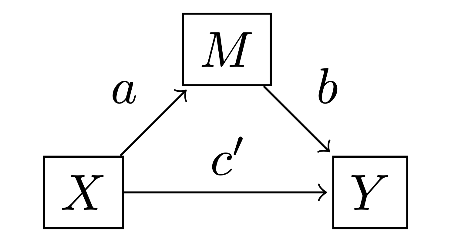
Using definitions from Hayes [2017], we can define a few effects of interest:

• Direct effect: is given by \(c'\). Two cases that differ by one unit on \(x\) but are equal on \(m\) are estimated to differ by \(c'\) units on \(y\).

• Indirect effect: is given by \(a \cdot b\). Two cases which differ by one unit of \(x\) are estimated to differ by \(a \cdot b\) units on \(y\) as a result of the effect of \(x \rightarrow m\) and \(m \rightarrow y\).

• Total effect: is \(c = c' + a \cdot b\) which is simply the sum of the direct and indirect effects. This could be understood as: two cases that differ by one unit on \(x\) are estimated to differ by \(a \cdot b\) units on \(y\) due to the indirect pathway \(x \rightarrow m \rightarrow y\), and by \(c'\) units due to the direct pathway \(x \rightarrow y\). The total effect could also be estimated by evaluating the alternative model \(y_i \sim \mathrm{Normal}(i_{Y*} + c \cdot x_i, \sigma_{Y*})\).

Generate simulated data

def make_data():
    N = 75
    a, b, cprime = 0.5, 0.6, 0.3
    im, iy, σm, σy = 2.0, 0.0, 0.5, 0.5
    x = rng.normal(loc=0, scale=1, size=N)
    m = im + rng.normal(loc=a * x, scale=σm, size=N)
    y = iy + (cprime * x) + rng.normal(loc=b * m, scale=σy, size=N)
    print(f"True direct effect = {cprime}")
    print(f"True indirect effect = {a*b}")
    print(f"True total effect = {cprime+a*b}")
    return x, m, y


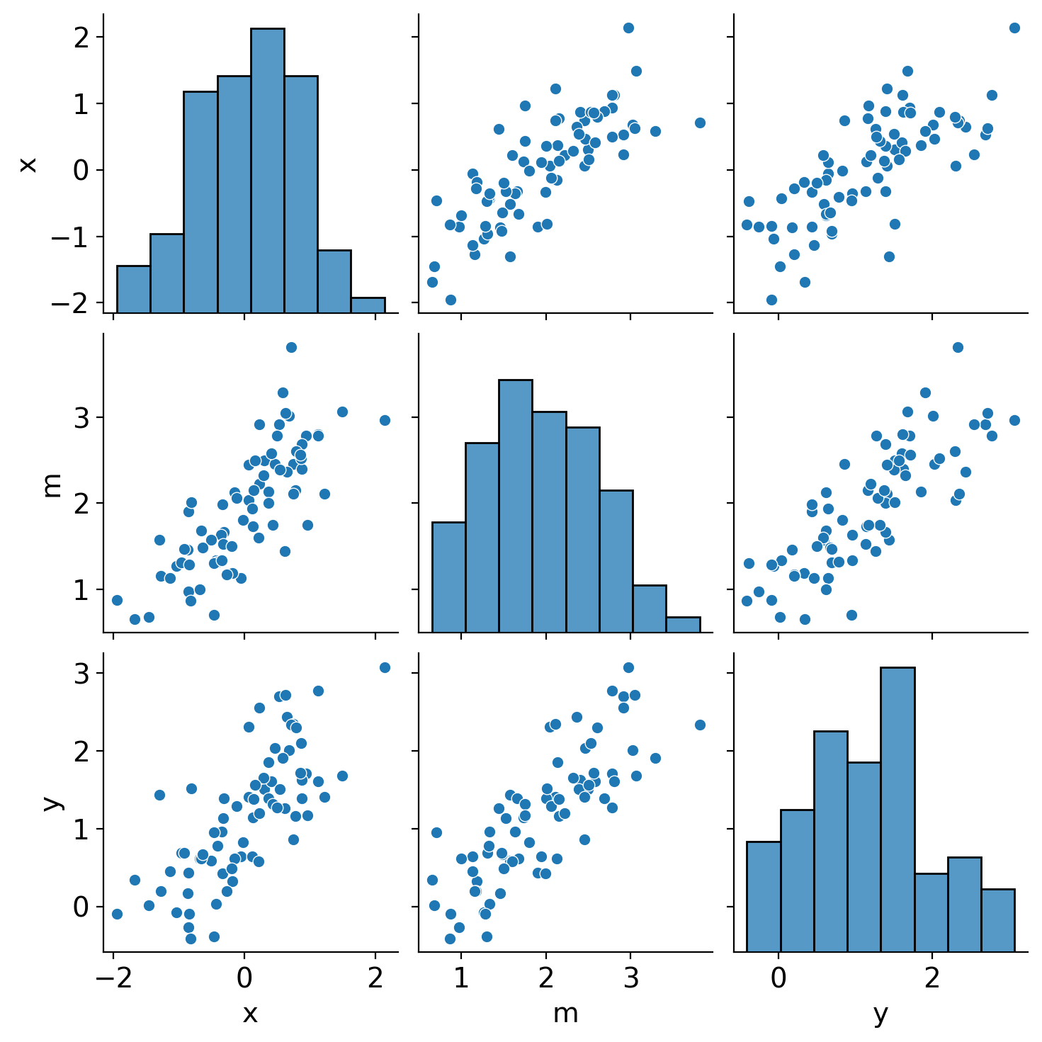
x, m, y = make_data()

sns.pairplot(DataFrame({"x": x, "m": m, "y": y}));

True direct effect = 0.3
True indirect effect = 0.3
True total effect = 0.6

Define the PyMC3 model and conduct inference

def mediation_model(x, m, y):
    with pm.Model() as model:
        x = pm.ConstantData("x", x, dims="obs_id")
        y = pm.ConstantData("y", y, dims="obs_id")
        m = pm.ConstantData("m", m, dims="obs_id")

        # intercept priors
        im = pm.Normal("im", mu=0, sigma=10)
        iy = pm.Normal("iy", mu=0, sigma=10)
        # slope priors
        a = pm.Normal("a", mu=0, sigma=10)
        b = pm.Normal("b", mu=0, sigma=10)
        cprime = pm.Normal("cprime", mu=0, sigma=10)
        # noise priors
        σm = pm.HalfCauchy("σm", 1)
        σy = pm.HalfCauchy("σy", 1)

        # likelihood
        pm.Normal("m_likelihood", mu=im + a * x, sigma=σm, observed=m, dims="obs_id")
        pm.Normal("y_likelihood", mu=iy + b * m + cprime * x, sigma=σy, observed=y, dims="obs_id")

        # calculate quantities of interest
        indirect_effect = pm.Deterministic("indirect effect", a * b)
        total_effect = pm.Deterministic("total effect", a * b + cprime)

    return model


model = mediation_model(x, m, y)
pm.model_to_graphviz(model)

with model:
    result = pm.sample(tune=4000, target_accept=0.9, random_seed=42)

Auto-assigning NUTS sampler...
Initializing NUTS using jitter+adapt_diag...
Multiprocess sampling (4 chains in 4 jobs)
NUTS: [im, iy, a, b, cprime, σm, σy]

100.00% [20000/20000 00:09<00:00 Sampling 4 chains, 0 divergences]

Sampling 4 chains for 4_000 tune and 1_000 draw iterations (16_000 + 4_000 draws total) took 9 seconds.

Visualise the trace to check for convergence.

az.plot_trace(result)
plt.tight_layout()

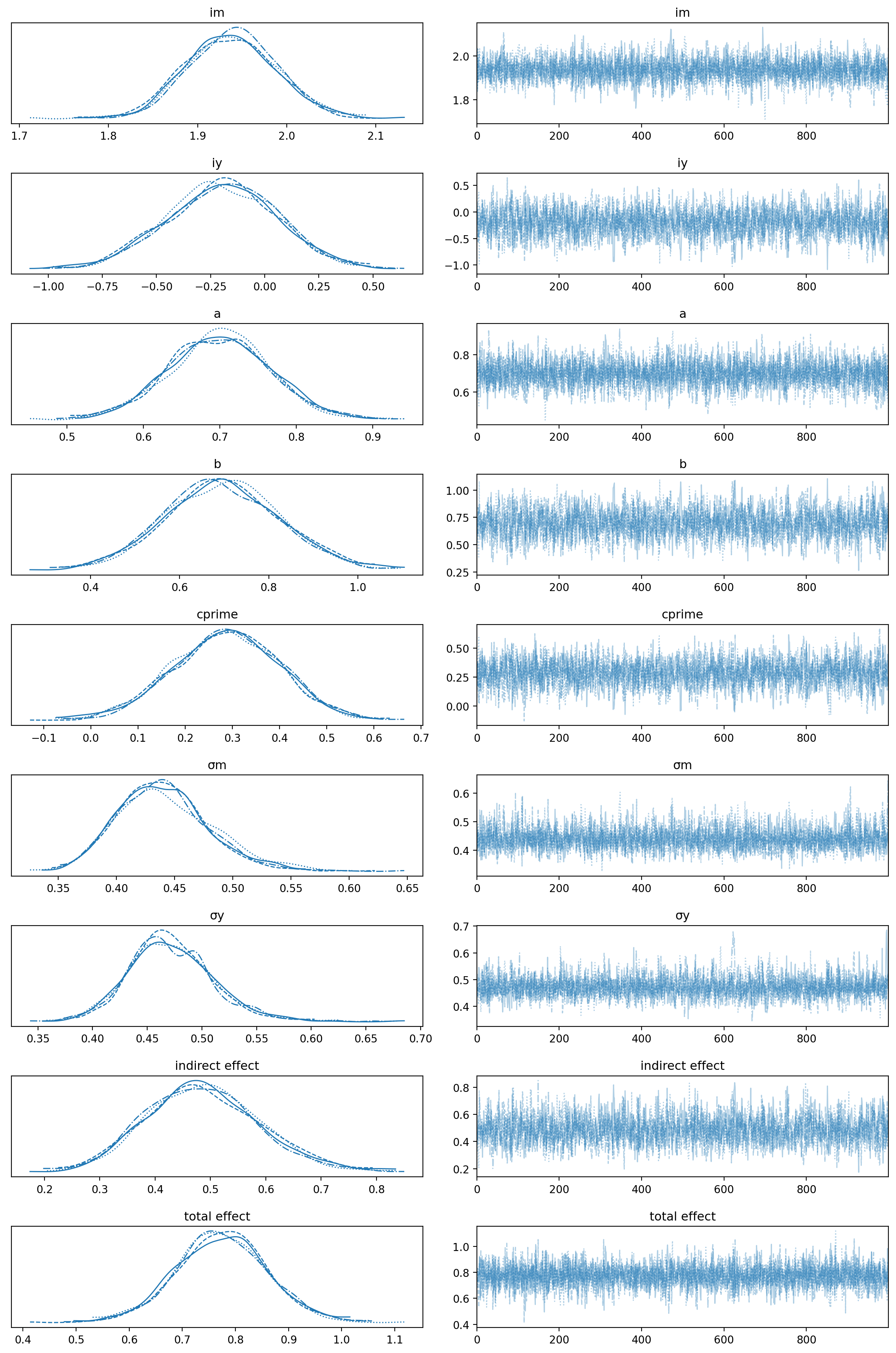
We have good chain mixing and the posteriors for each chain look very similar, so no problems in that regard.

Visualise the important parameters

First we will use a pair plot to look at joint posterior distributions.

az.plot_pair(
    result,
    marginals=True,
    point_estimate="median",
    figsize=(12, 12),
    scatter_kwargs={"alpha": 0.05},
    var_names=["a", "b", "cprime", "indirect effect", "total effect"],
);

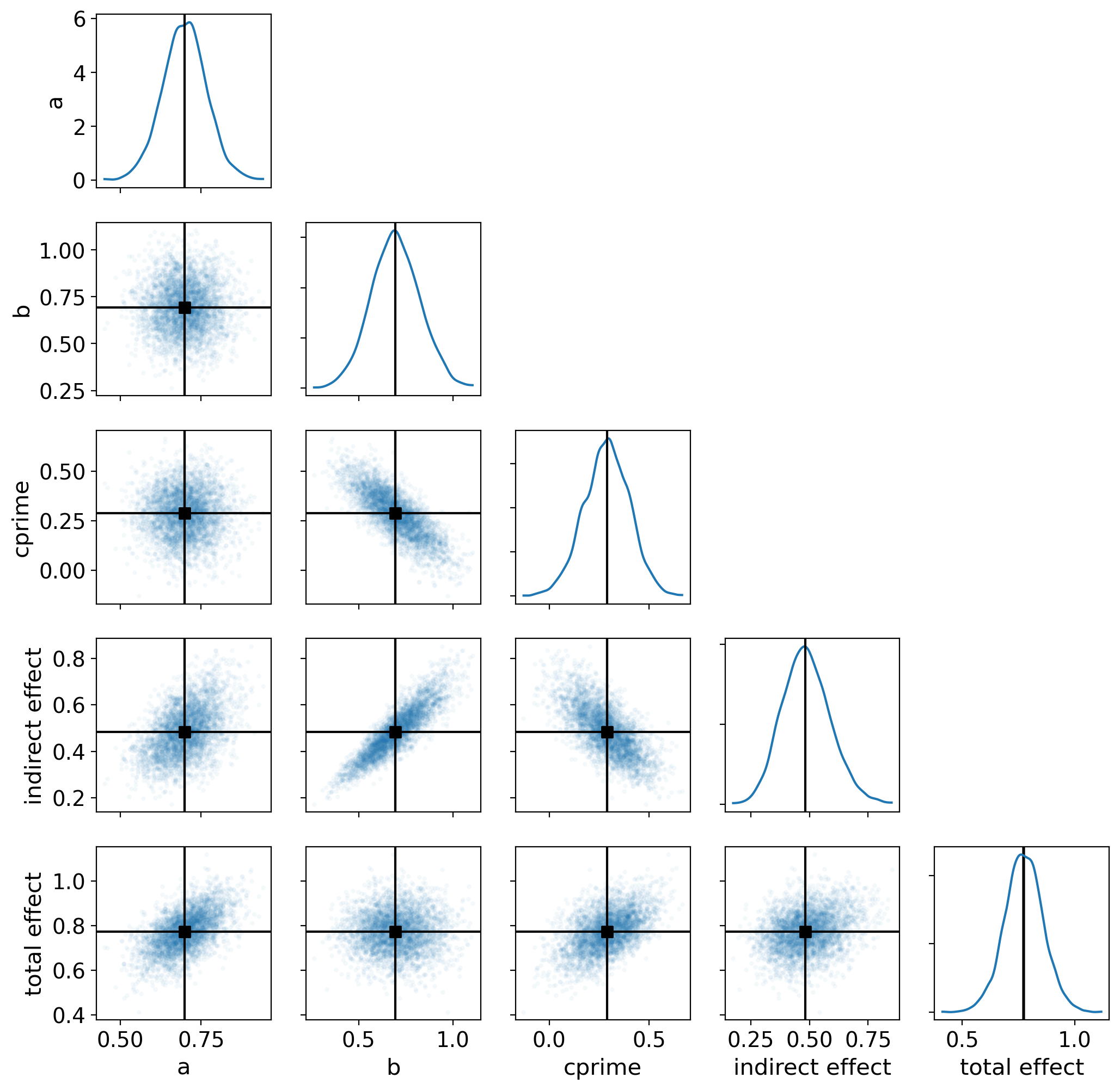
Interpreting the results

We can take a closer look at the indirect, total, and direct effects:

ax = az.plot_posterior(
    result,
    var_names=["cprime", "indirect effect", "total effect"],
    ref_val=0,
    hdi_prob=0.95,
    figsize=(14, 4),
)
ax[0].set(title="direct effect");

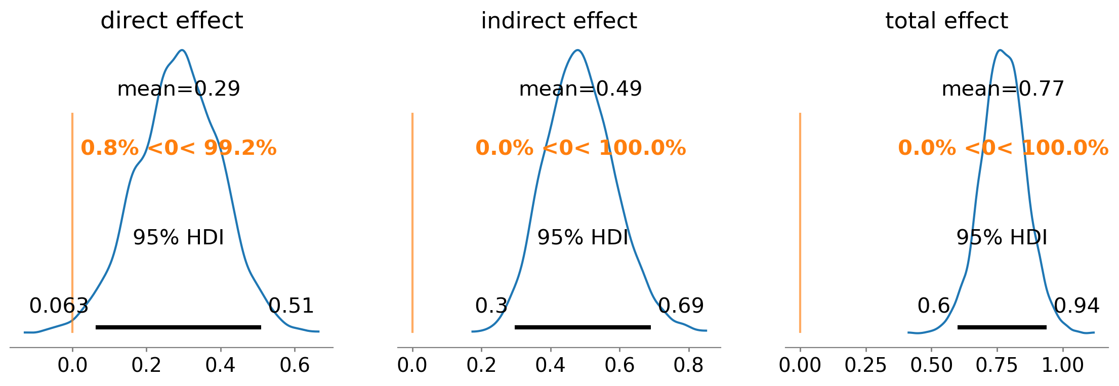
• The posterior mean direct effect is 0.29, meaning that for every 1 unit of increase in \(x\), \(y\) increases by 0.29 due to the direct effect \(x \rightarrow y\).

• The posterior mean indirect effect is 0.49, meaning that for every 1 unit of increase in \(x\), \(y\) increases by 0.49 through the pathway \(x \rightarrow m \rightarrow y\). The probability that the indirect effect is zero is infinitesimal.

• The posterior mean total effect is 0.77, meaning that for every 1 unit of increase in \(x\), \(y\) increases by 0.77 through both the direct and indirect pathways.

Double check with total effect only model

Above, we stated that the total effect could also be estimated by evaluating the alternative model \(y_i \sim \mathrm{Normal}(i_{Y*} + c \cdot x_i, \sigma_{Y*})\). Here we will check this by comparing the posterior distribution for \(c'\) in the mediation model, and the posterior distribution for \(c\) in this alternative model.

with pm.Model() as total_effect_model:
    _x = pm.ConstantData("_x", x, dims="obs_id")
    iy = pm.Normal("iy", mu=0, sigma=1)
    c = pm.Normal("c", mu=0, sigma=1)
    σy = pm.HalfCauchy("σy", 1)
    μy = iy + c * _x
    pm.Normal("yy", mu=μy, sigma=σy, observed=y, dims="obs_id")

with total_effect_model:
    total_effect_result = pm.sample(tune=4000, target_accept=0.9, random_seed=42)

Auto-assigning NUTS sampler...
Initializing NUTS using jitter+adapt_diag...
Multiprocess sampling (4 chains in 4 jobs)
NUTS: [iy, c, σy]

100.00% [20000/20000 00:01<00:00 Sampling 4 chains, 0 divergences]

Sampling 4 chains for 4_000 tune and 1_000 draw iterations (16_000 + 4_000 draws total) took 2 seconds.

fig, ax = plt.subplots(figsize=(14, 4))
az.plot_posterior(
    total_effect_result, var_names=["c"], point_estimate=None, hdi_prob="hide", c="r", lw=4, ax=ax
)
az.plot_posterior(
    result, var_names=["total effect"], point_estimate=None, hdi_prob="hide", c="k", lw=4, ax=ax
);

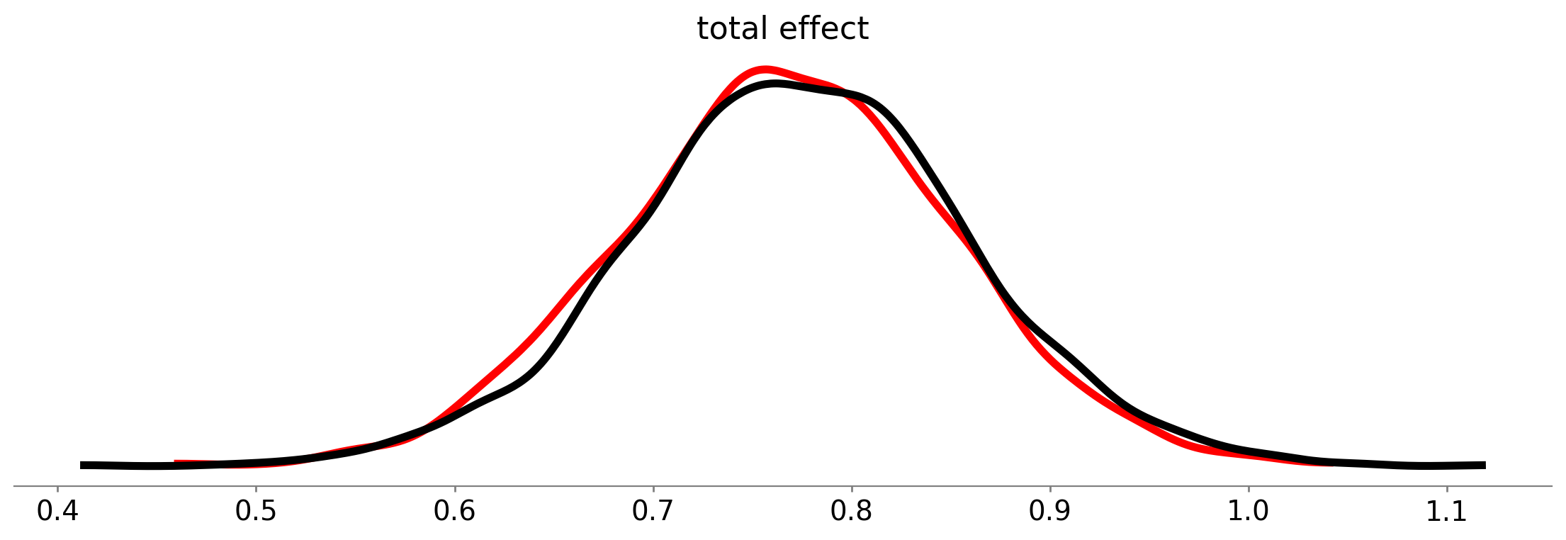
As we can see, the posterior distributions over the direct effects are near-identical for the mediation model (black curve) and the direct model (red curve).

Parameter estimation versus hypothesis testing

This notebook has focused on the approach of Bayesian parameter estimation. For many situations this is entirely sufficient, and more information can be found in Yuan and MacKinnon [2009]. It will tell us, amongst other things, what our posterior beliefs are in the direct effects, indirect effects, and total effects. And we can use those posterior beliefs to conduct posterior predictive checks to visually check how well the model accounts for the data.

However, depending upon the use case it may be preferable to test hypotheses about the presence or absence of an indirect effect (\(x \rightarrow m \rightarrow y\)) for example. In this case, it may be more appropriate to take a more explicit hypothesis testing approach to see examine the relative credibility of the mediation model as compared to a simple direct effect model (i.e. \(y_i = \mathrm{Normal}(i_{Y*} + c \cdot x_i, \sigma_{Y*})\)). Readers are referred to Nuijten et al. [2015] for a hypothesis testing approach to Bayesian mediation models and to Kruschke [2011] for more information on parameter estimation versus hypothesis testing.

Summary

As stated at the outset, the procedures used in mediation analysis have evolved over time. So there are plenty of people who are not necessarily up to speed with modern best practice. The approach in this notebook sticks to that outlined by Hayes [2017], but it is relevant to be aware of some of this history to avoid confusion - which is particularly important if defending your approach in peer review.

Authors

• Authored by Benjamin T. Vincent in August 2021

• Updated by Benjamin T. Vincent in February 2022

References

[1] (1,2,3)

Andrew F Hayes. Introduction to mediation, moderation, and conditional process analysis: A regression-based approach. Guilford publications, 2017.

[2]

Ying Yuan and David P MacKinnon. Bayesian mediation analysis. Psychological methods, 14(4):301, 2009.

[3]

Michèle B Nuijten, Ruud Wetzels, Dora Matzke, Conor V Dolan, and Eric-Jan Wagenmakers. A default bayesian hypothesis test for mediation. Behavior research methods, 47(1):85–97, 2015.

[4]

John K Kruschke. Bayesian assessment of null values via parameter estimation and model comparison. Perspectives on Psychological Science, 6(3):299–312, 2011.

Watermark

%load_ext watermark
%watermark -n -u -v -iv -w -p pytensor,aeppl,xarray

Last updated: Wed Feb 01 2023

Python implementation: CPython
Python version       : 3.11.0
IPython version      : 8.9.0

pytensor: 2.8.11
aeppl   : not installed
xarray  : 2023.1.0

arviz     : 0.14.0
pymc      : 5.0.1
matplotlib: 3.6.3
numpy     : 1.24.1
seaborn   : 0.12.2

Watermark: 2.3.1

License notice

All the notebooks in this example gallery are provided under the MIT License which allows modification, and redistribution for any use provided the copyright and license notices are preserved.

Citing PyMC examples

To cite this notebook, use the DOI provided by Zenodo for the pymc-examples repository.

Important

Many notebooks are adapted from other sources: blogs, books… In such cases you should cite the original source as well.

Also remember to cite the relevant libraries used by your code.

Here is an citation template in bibtex:

@incollection{citekey,
  author    = "<notebook authors, see above>",
  title     = "<notebook title>",
  editor    = "PyMC Team",
  booktitle = "PyMC examples",
  doi       = "10.5281/zenodo.5654871"
}

which once rendered could look like: