Introduction to Variational Inference with PyMC

The most common strategy for computing posterior quantities of Bayesian models is via sampling, particularly Markov chain Monte Carlo (MCMC) algorithms. While sampling algorithms and associated computing have continually improved in performance and efficiency, MCMC methods still scale poorly with data size, and become prohibitive for more than a few thousand observations. A more scalable alternative to sampling is variational inference (VI), which re-frames the problem of computing the posterior distribution as an optimization problem.

In PyMC, the variational inference API is focused on approximating posterior distributions through a suite of modern algorithms. Common use cases to which this module can be applied include:

• Sampling from model posterior and computing arbitrary expressions

• Conducting Monte Carlo approximation of expectation, variance, and other statistics

• Removing symbolic dependence on PyMC random nodes and evaluate expressions (using eval)

• Providing a bridge to arbitrary PyTensor code

import arviz as az
import matplotlib.pyplot as plt
import numpy as np
import pymc as pm
import pytensor
import seaborn as sns

np.random.seed(42)

az.style.use("arviz-variat")

Distributional Approximations

There are severa methods in statistics that use a simpler distribution to approximate a more complex distribution. Perhaps the best-known example is the Laplace (normal) approximation. This involves constructing a Taylor series of the target posterior, but retaining only the terms of quadratic order and using those to construct a multivariate normal approximation.

Similarly, variational inference is another distributional approximation method where, rather than leveraging a Taylor series, some class of approximating distribution is chosen and its parameters are optimized such that the resulting distribution is as close as possible to the posterior. In essence, VI is a deterministic approximation that places bounds on the density of interest, then uses opimization to choose from that bounded set.

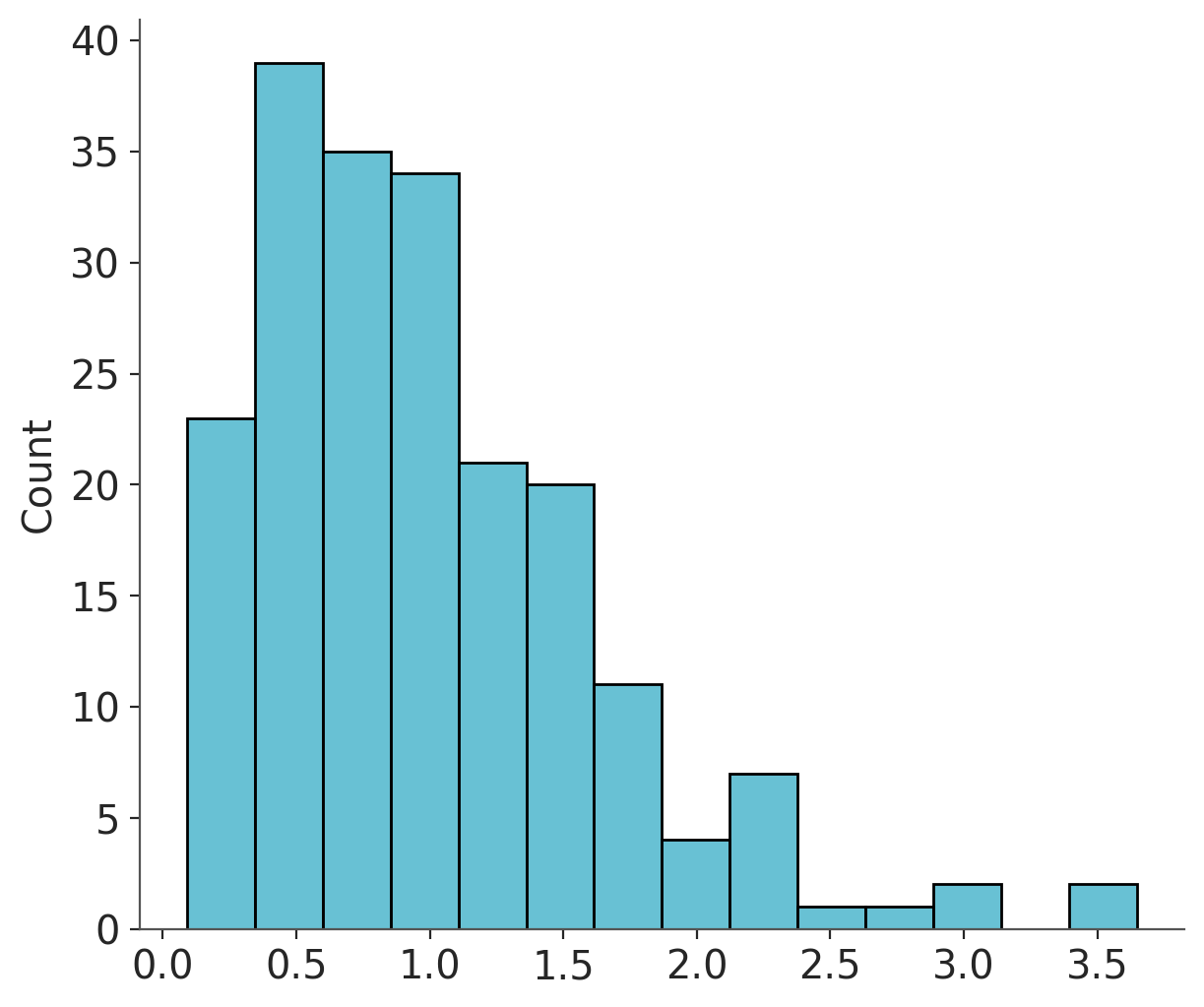
gamma_data = np.random.gamma(2, 0.5, size=200)
sns.histplot(gamma_data);

with pm.Model() as gamma_model:
    alpha = pm.Exponential("alpha", 0.1)
    beta = pm.Exponential("beta", 0.1)

    y = pm.Gamma("y", alpha, beta, observed=gamma_data)

with gamma_model:
    # mean_field = pm.fit()
    mean_field = pm.fit(obj_optimizer=pm.adagrad_window(learning_rate=1e-2))

Finished [100%]: Average Loss = 169.86

with gamma_model:
    trace = pm.sample()

Initializing NUTS using jitter+adapt_diag...

Multiprocess sampling (4 chains in 4 jobs)

NUTS: [alpha, beta]

Sampling 4 chains for 1_000 tune and 1_000 draw iterations (4_000 + 4_000 draws total) took 1 seconds.

mean_field

<pymc.variational.approximations.MeanField at 0x126cd4560>

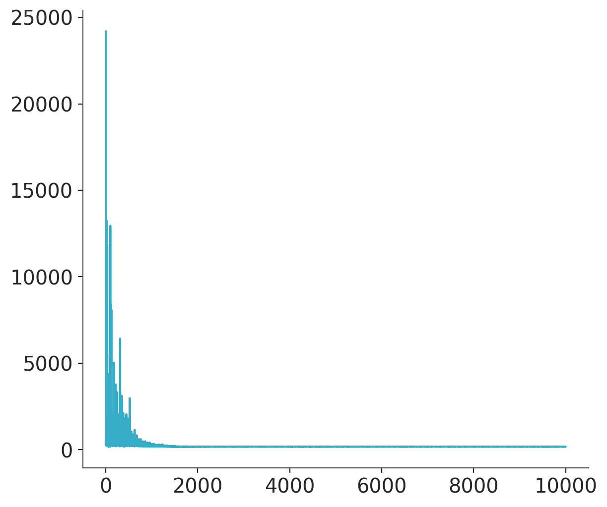
plt.plot(mean_field.hist);

with gamma_model:
    approx_sample = mean_field.sample(1000)

with gamma_model:
    approx_sample = mean_field.sample(1000)
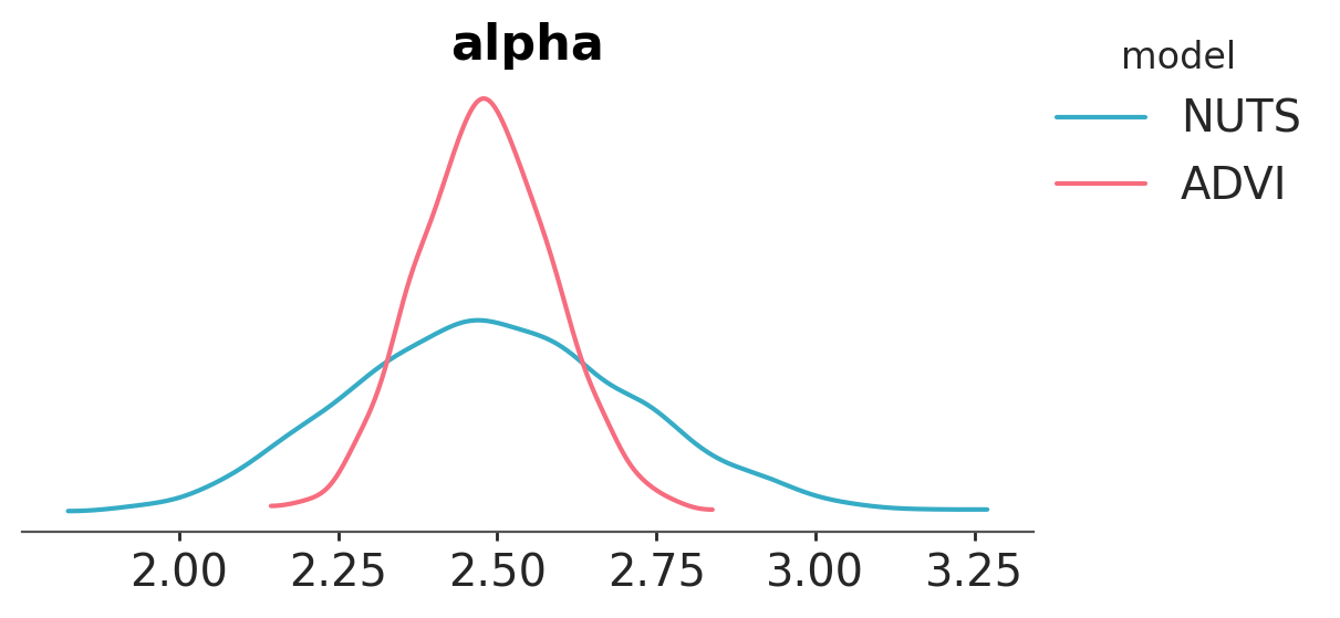
pc = az.plot_dist(
    {"NUTS": trace, "ADVI": approx_sample},
    var_names=["alpha"],
    visuals={
        "credible_interval": False,
        "point_estimate": False,
        "point_estimate_text": False,
    },
)
pc.add_legend("model");

/Users/ethanyang/Developer/github.com/pymc-devs/pymc/.venv/lib/python3.12/site-packages/arviz_plots/plot_collection.py:56: FutureWarning: In a future version of xarray the default value for join will change from join='outer' to join='exact'. This change will result in the following ValueError: cannot be aligned with join='exact' because index/labels/sizes are not equal along these coordinates (dimensions): 'chain' ('chain',) The recommendation is to set join explicitly for this case.
  data = xr.concat(ds_list, dim="model").assign_coords(model=list(data))

Basic setup

We do not need complex models to play with the VI API; let’s begin with a simple mixture model:

w = np.array([0.2, 0.8])
mu = np.array([-0.3, 0.5])
sd = np.array([0.1, 0.1])

with pm.Model() as model:
    x = pm.NormalMixture("x", w=w, mu=mu, sigma=sd)
    x2 = x**2
    sin_x = pm.math.sin(x)

We can’t compute analytical expectations for this model. However, we can obtain an approximation using Markov chain Monte Carlo methods; let’s use NUTS first.

To allow samples of the expressions to be saved, we need to wrap them in Deterministic objects:

with model:
    pm.Deterministic("x2", x2)
    pm.Deterministic("sin_x", sin_x)

with model:
    trace = pm.sample(5000)

Initializing NUTS using jitter+adapt_diag...

Multiprocess sampling (4 chains in 4 jobs)

NUTS: [x]

Sampling 4 chains for 1_000 tune and 5_000 draw iterations (4_000 + 20_000 draws total) took 2 seconds.

There were 487 divergences after tuning. Increase `target_accept` or reparameterize.

The rhat statistic is larger than 1.01 for some parameters. This indicates problems during sampling. See https://arxiv.org/abs/1903.08008 for details

The effective sample size per chain is smaller than 100 for some parameters.  A higher number is needed for reliable rhat and ess computation. See https://arxiv.org/abs/1903.08008 for details

az.plot_trace_dist(trace);

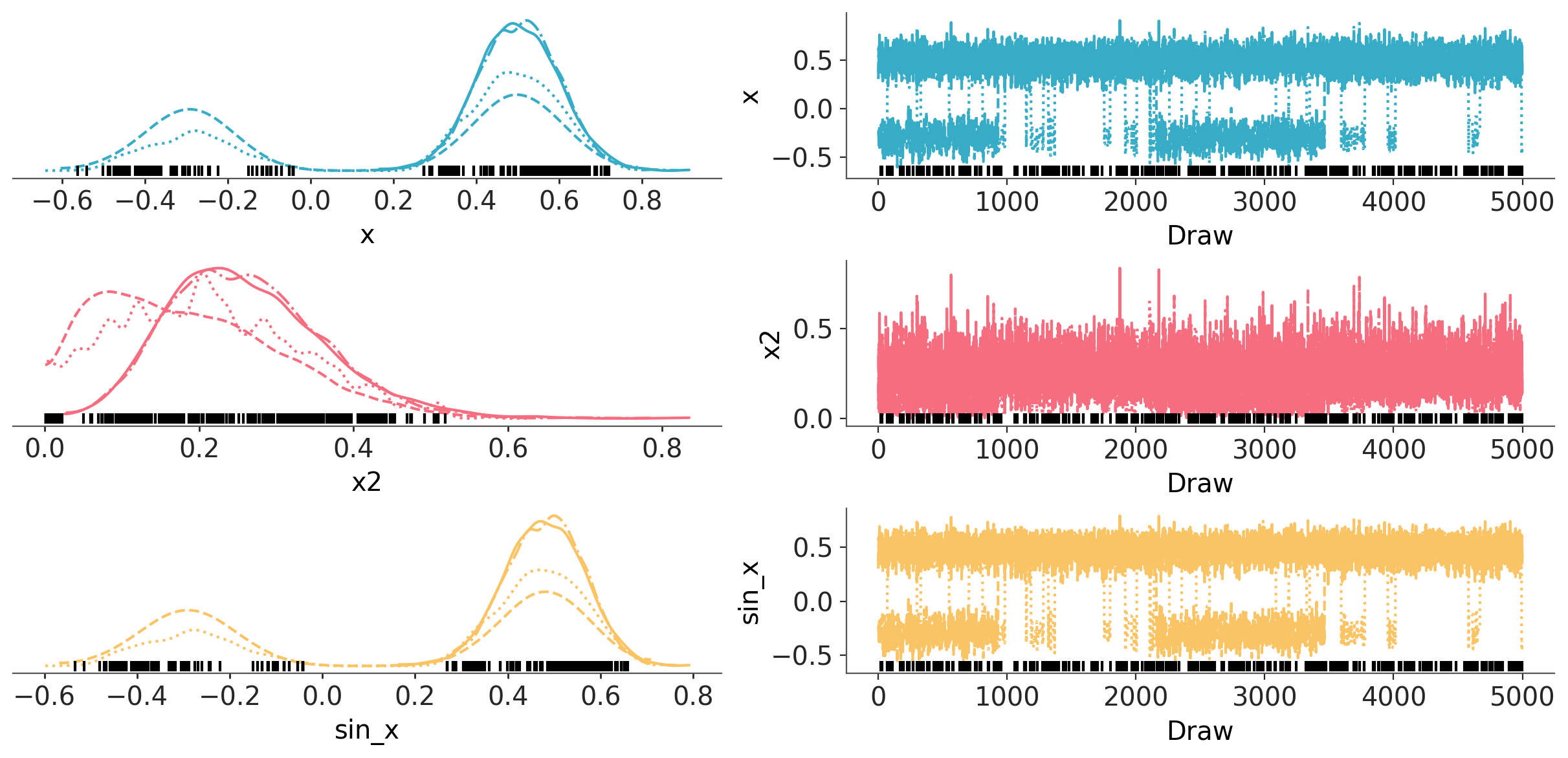
Above are traces for \(x^2\) and \(sin(x)\). We can see there is clear multi-modality in this model. One drawback, is that you need to know in advance what exactly you want to see in trace and wrap it with Deterministic.

The VI API takes an alternate approach: You obtain inference from model, then calculate expressions based on this model afterwards.

Let’s use the same model:

with pm.Model() as model:
    x = pm.NormalMixture("x", w=w, mu=mu, sigma=sd)
    x2 = x**2
    sin_x = pm.math.sin(x)

Here we will use automatic differentiation variational inference (ADVI).

with model:
    mean_field = pm.fit(method="advi")

Finished [100%]: Average Loss = 2.1689

with model:
    posterior_sample = mean_field.sample(1000)
az.plot_dist(posterior_sample, var_names=["x"]);

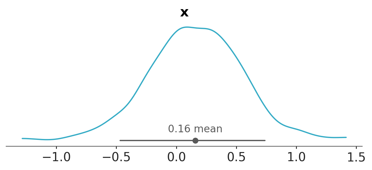
Notice that ADVI has failed to approximate the multimodal distribution, since it uses a Gaussian distribution that has a single mode.

Checking convergence

Let’s use the default arguments for CheckParametersConvergence as they seem to be reasonable.

from pymc.variational.callbacks import CheckParametersConvergence

with model:
    mean_field = pm.fit(method="advi", callbacks=[CheckParametersConvergence()])

Convergence achieved at 7600

Interrupted at 7,599 [75%]: Average Loss = 3.89

We can access inference history via .hist attribute.

plt.plot(mean_field.hist);

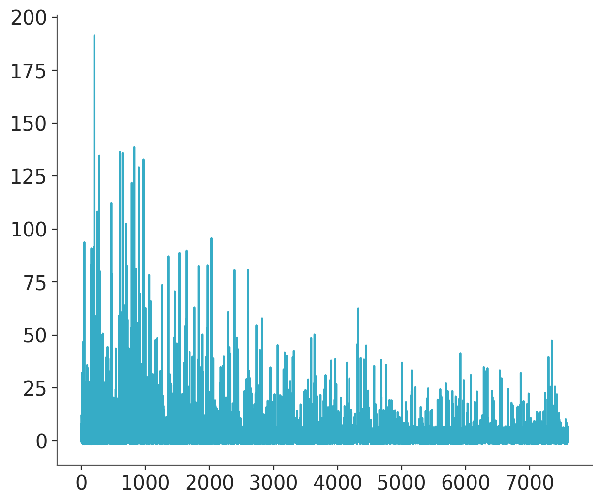
This is not a good convergence plot, despite the fact that we ran many iterations. The reason is that the mean of the ADVI approximation is close to zero, and therefore taking the relative difference (the default method) is unstable for checking convergence.

with model:
    mean_field = pm.fit(
        method="advi",
        callbacks=[pm.variational.callbacks.CheckParametersConvergence(diff="absolute")],
    )

Convergence achieved at 7600

Interrupted at 7,599 [75%]: Average Loss = 3.9735

plt.plot(mean_field.hist);

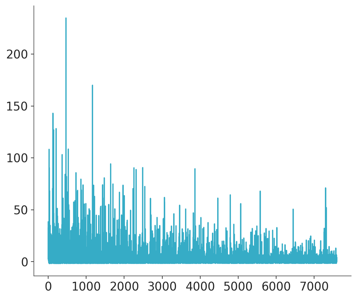
That’s much better! We’ve reached convergence after less than 5000 iterations.

Tracking parameters

Another useful callback allows users to track parameters. It allows for the tracking of arbitrary statistics during inference, though it can be memory-hungry. Using the fit function, we do not have direct access to the approximation before inference. However, tracking parameters requires access to the approximation. We can get around this constraint by using the object-oriented (OO) API for inference.

with model:
    advi = pm.ADVI()

advi.approx;

Different approximations have different hyperparameters. In mean-field ADVI, we have \(\rho\) and \(\mu\) (inspired by Bayes by BackProp).

advi.approx.shared_params

{'mu': mu, 'rho': rho}

There are convenient shortcuts to relevant statistics associated with the approximation. This can be useful, for example, when specifying a mass matrix for NUTS sampling:

advi.approx.mean.eval(), advi.approx.std.eval()

(array([0.34]), array([0.69314718]))

We can roll these statistics into the Tracker callback.

tracker = pm.variational.callbacks.Tracker(
    mean=advi.approx.mean.eval,  # callable that returns mean
    std=advi.approx.std.eval,  # callable that returns std
)

Now, calling advi.fit will record the mean and standard deviation of the approximation as it runs.

approx = advi.fit(20000, callbacks=[tracker])

Finished [100%]: Average Loss = 1.969

We can now plot both the evidence lower bound and parameter traces:

fig = plt.figure(figsize=(16, 9))
mu_ax = fig.add_subplot(221)
std_ax = fig.add_subplot(222)
hist_ax = fig.add_subplot(212)
mu_ax.plot(tracker["mean"])
mu_ax.set_title("Mean track")
std_ax.plot(tracker["std"])
std_ax.set_title("Std track")
hist_ax.plot(advi.hist)
hist_ax.set_title("Negative ELBO track");

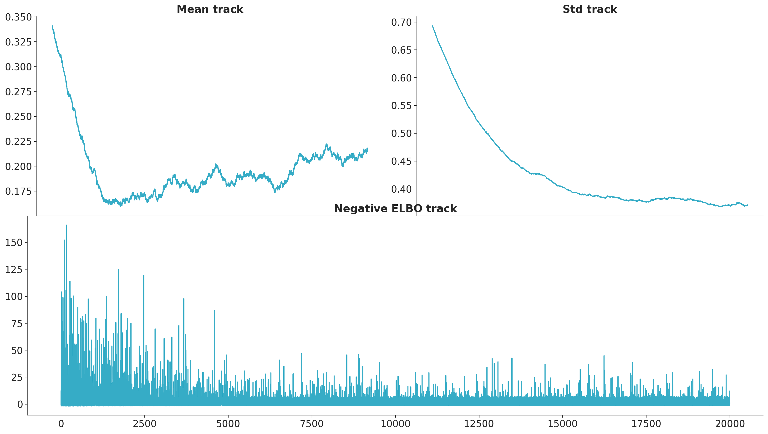
Notice that there are convergence issues with the mean, and that lack of convergence does not seem to change the ELBO trajectory significantly. As we are using the OO API, we can run the approximation longer until convergence is achieved.

advi.refine(100_000)

Finished [100%]: Average Loss = 2.0239

Let’s take a look:

fig = plt.figure(figsize=(16, 9))
mu_ax = fig.add_subplot(221)
std_ax = fig.add_subplot(222)
hist_ax = fig.add_subplot(212)
mu_ax.plot(tracker["mean"])
mu_ax.set_title("Mean track")
std_ax.plot(tracker["std"])
std_ax.set_title("Std track")
hist_ax.plot(advi.hist)
hist_ax.set_title("Negative ELBO track");

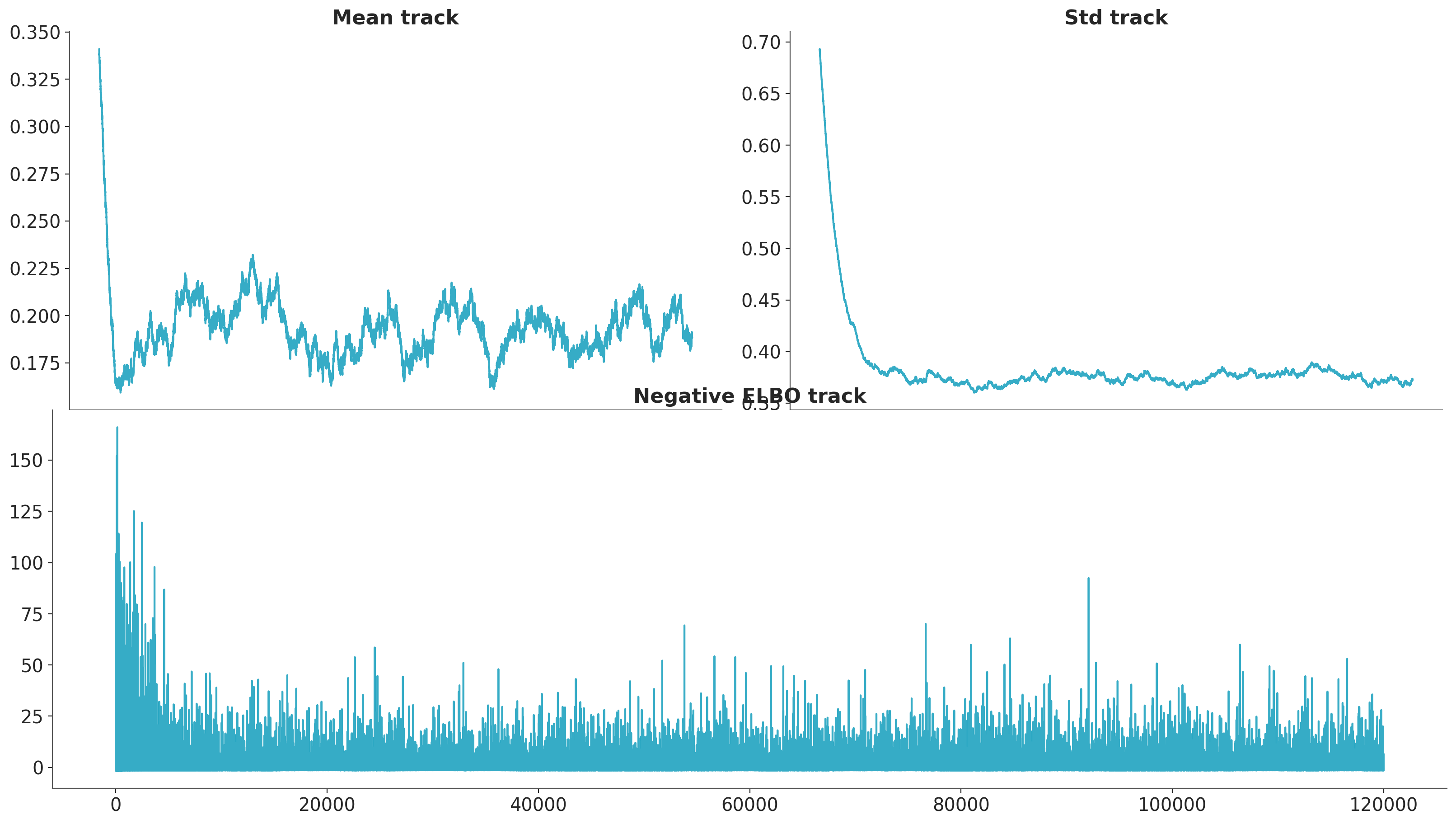
We still see evidence for lack of convergence, as the mean has devolved into a random walk. This could be the result of choosing a poor algorithm for inference. At any rate, it is unstable and can produce very different results even using different random seeds.

Let’s compare results with the NUTS output:

with model:
    advi_sample = approx.sample(20000)
pc = az.plot_dist(
    {"NUTS": trace, "ADVI": advi_sample},
    var_names=["x"],
    visuals={
        "credible_interval": False,
        "point_estimate": False,
        "point_estimate_text": False,
    },
)
pc.add_legend("model");

/Users/ethanyang/Developer/github.com/pymc-devs/pymc/.venv/lib/python3.12/site-packages/arviz_plots/plot_collection.py:56: FutureWarning: In a future version of xarray the default value for join will change from join='outer' to join='exact'. This change will result in the following ValueError: cannot be aligned with join='exact' because index/labels/sizes are not equal along these coordinates (dimensions): 'chain' ('chain',) The recommendation is to set join explicitly for this case.
  data = xr.concat(ds_list, dim="model").assign_coords(model=list(data))
/Users/ethanyang/Developer/github.com/pymc-devs/pymc/.venv/lib/python3.12/site-packages/arviz_plots/plot_collection.py:56: FutureWarning: In a future version of xarray the default value for join will change from join='outer' to join='exact'. This change will result in the following ValueError: cannot be aligned with join='exact' because index/labels/sizes are not equal along these coordinates (dimensions): 'draw' ('draw',) The recommendation is to set join explicitly for this case.
  data = xr.concat(ds_list, dim="model").assign_coords(model=list(data))

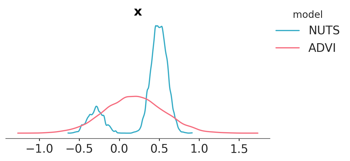
Again, we see that ADVI is not able to cope with multimodality; we can instead use SVGD, which generates an approximation based on a large number of particles.

with model:
    svgd_approx = pm.fit(
        300,
        method="svgd",
        inf_kwargs=dict(n_particles=1000),
        obj_optimizer=pm.sgd(learning_rate=0.01),
    )

with model:
    advi_sample = approx.sample(10000)
    svgd_sample = svgd_approx.sample(2000)
pc = az.plot_dist(
    {"NUTS": trace, "ADVI": advi_sample, "SVGD": svgd_sample},
    var_names=["x"],
    visuals={
        "credible_interval": False,
        "point_estimate": False,
        "point_estimate_text": False,
    },
)
pc.add_legend("model");

/Users/ethanyang/Developer/github.com/pymc-devs/pymc/.venv/lib/python3.12/site-packages/arviz_plots/plot_collection.py:56: FutureWarning: In a future version of xarray the default value for join will change from join='outer' to join='exact'. This change will result in the following ValueError: cannot be aligned with join='exact' because index/labels/sizes are not equal along these coordinates (dimensions): 'chain' ('chain',) The recommendation is to set join explicitly for this case.
  data = xr.concat(ds_list, dim="model").assign_coords(model=list(data))
/Users/ethanyang/Developer/github.com/pymc-devs/pymc/.venv/lib/python3.12/site-packages/arviz_plots/plot_collection.py:56: FutureWarning: In a future version of xarray the default value for join will change from join='outer' to join='exact'. This change will result in the following ValueError: cannot be aligned with join='exact' because index/labels/sizes are not equal along these coordinates (dimensions): 'draw' ('draw',) The recommendation is to set join explicitly for this case.
  data = xr.concat(ds_list, dim="model").assign_coords(model=list(data))

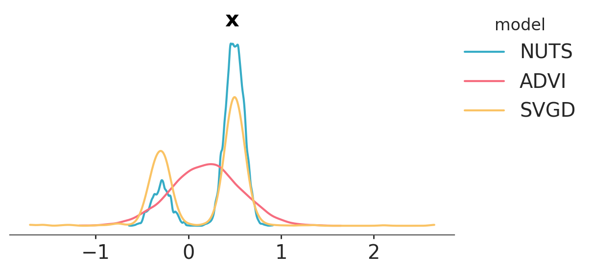
That did the trick, as we now have a multimodal approximation using SVGD.

With this, it is possible to calculate arbitrary functions of the parameters with this variational approximation. For example we can calculate \(x^2\) and \(sin(x)\), as with the NUTS model.

# recall x ~ NormalMixture
a = x**2
b = pm.math.sin(x)

To evaluate these expressions with the approximation, we need approx.sample_node.

a_sample = svgd_approx.sample_node(a)
a_sample.eval()

array(0.12755756)

a_sample.eval()

array(0.12755756)

a_sample.eval()

array(0.12755756)

Note: repeated .eval() calls on the same sample_node produce the same draw because PyTensor’s compiled function reads the shared RNG state but does not advance it between calls. To get fresh independent samples, use sample_node(node, size=N), which materializes N draws within a single graph evaluation.

By applying replacements, sample_node swaps the model’s random variables for draws from the approximation. The expression still builds on the model, but its randomness now comes from the approximation, so changing the approximation changes the distribution of the stochastic nodes.

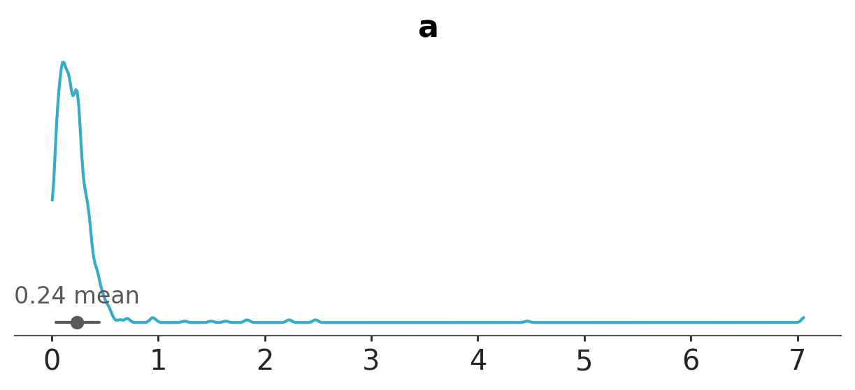
a_dataset = az.convert_to_dataset({"a": svgd_approx.sample_node(a, size=2000).eval()[None, :]})
az.plot_dist(a_dataset, var_names=["a"]);

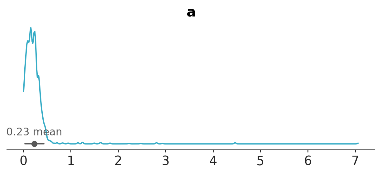
There is a more convenient way to get lots of samples at once: sample_node

a_samples = svgd_approx.sample_node(a, size=1000)

a_dataset = az.convert_to_dataset({"a": a_samples.eval()[None, :]})
az.plot_dist(a_dataset, var_names=["a"]);

The sample_node function includes an additional dimension, so taking expectations or calculating variance is specified by axis=0.

a_samples.var(0).eval()  # variance

array(0.15712698)

a_samples.mean(0).eval()  # mean

array(0.23765686)

A symbolic sample size can also be specified:

import pytensor.tensor as pt

i = pt.iscalar("i")
i.tag.test_value = 1
a_samples_i = svgd_approx.sample_node(a, size=i)

a_samples_i.eval({i: 100}).shape

(100,)

a_samples_i.eval({i: 10000}).shape

(10000,)

Unfortunately the size must be a scalar value.

Multilabel logistic regression

Let’s illustrate the use of Tracker with the famous Iris dataset. We’ll attempy multi-label classification and compute the expected accuracy score as a diagnostic.

import pandas as pd

from sklearn.datasets import load_iris
from sklearn.model_selection import train_test_split

X, y = load_iris(return_X_y=True)
X_train, X_test, y_train, y_test = train_test_split(X, y)

A relatively simple model will be sufficient here because the classes are roughly linearly separable; we are going to fit multinomial logistic regression.

Xt = pytensor.shared(X_train)
yt = pytensor.shared(y_train)

with pm.Model() as iris_model:
    # Coefficients for features
    β = pm.Normal("β", 0, sigma=1e2, shape=(4, 3))
    # Transoform to unit interval
    a = pm.Normal("a", sigma=1e4, shape=(3,))
    p = pt.special.softmax(Xt.dot(β) + a, axis=-1)

    observed = pm.Categorical("obs", p=p, observed=yt)

Applying replacements in practice

PyMC models have symbolic inputs for latent variables. To evaluate an expression that requires knowledge of latent variables, one needs to provide fixed values. We can use values approximated by VI for this purpose. The function sample_node removes the symbolic dependencies.

sample_node will use the whole distribution at each step, so we will use it here. We can apply more replacements in single function call using the more_replacements keyword argument in both replacement functions.

HINT: You can use more_replacements argument when calling fit too:

• pm.fit(more_replacements={full_data: minibatch_data})

• inference.fit(more_replacements={full_data: minibatch_data})

with iris_model:
    # We'll use SVGD
    inference = pm.SVGD(n_particles=500, jitter=1)

    # Local reference to approximation
    approx = inference.approx

    # Here we need `more_replacements` to change train_set to test_set
    test_probs = approx.sample_node(p, more_replacements={Xt: X_test}, size=100)

    # For train set no more replacements needed
    train_probs = approx.sample_node(p)

By applying the code above, we now have 100 sampled probabilities (default number for sample_node is None) for each observation.

Next we create symbolic expressions for sampled accuracy scores:

test_ok = pt.eq(test_probs.argmax(-1), y_test)
train_ok = pt.eq(train_probs.argmax(-1), y_train)
test_accuracy = test_ok.mean(-1)
train_accuracy = train_ok.mean(-1)

Tracker expects callables so we can pass .eval method of PyTensor node that is function itself.

Calls to this function are cached so they can be reused.

eval_tracker = pm.variational.callbacks.Tracker(
    test_accuracy=test_accuracy.eval, train_accuracy=train_accuracy.eval
)

inference.fit(100, callbacks=[eval_tracker]);

_, ax = plt.subplots(1, 1)
df = pd.DataFrame(eval_tracker["test_accuracy"]).T.melt()
sns.lineplot(x="variable", y="value", data=df, color="red", ax=ax)
ax.plot(eval_tracker["train_accuracy"], color="blue")
ax.set_xlabel("epoch")
plt.legend(["test_accuracy", "train_accuracy"])
plt.title("Training Progress");

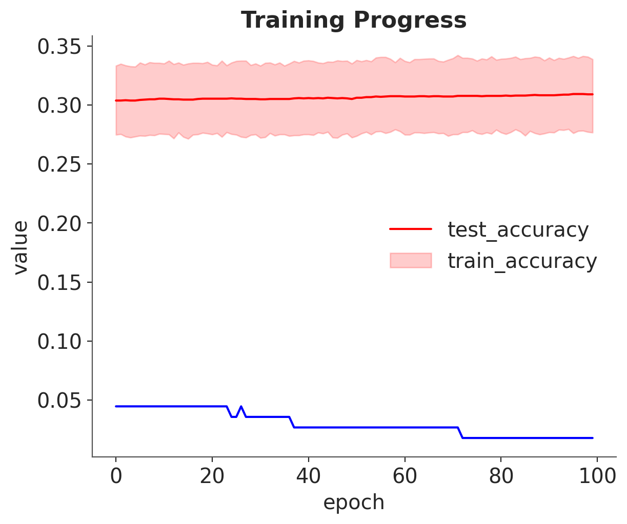
Training does not seem to be working here. Let’s use a different optimizer and boost the learning rate.

inference.fit(400, obj_optimizer=pm.adamax(learning_rate=0.1), callbacks=[eval_tracker]);

_, ax = plt.subplots(1, 1)
df = pd.DataFrame(np.asarray(eval_tracker["test_accuracy"])).T.melt()
sns.lineplot(x="variable", y="value", data=df, color="red", ax=ax)
ax.plot(eval_tracker["train_accuracy"], color="blue")
ax.set_xlabel("epoch")
plt.legend(["test_accuracy", "train_accuracy"])
plt.title("Training Progress");

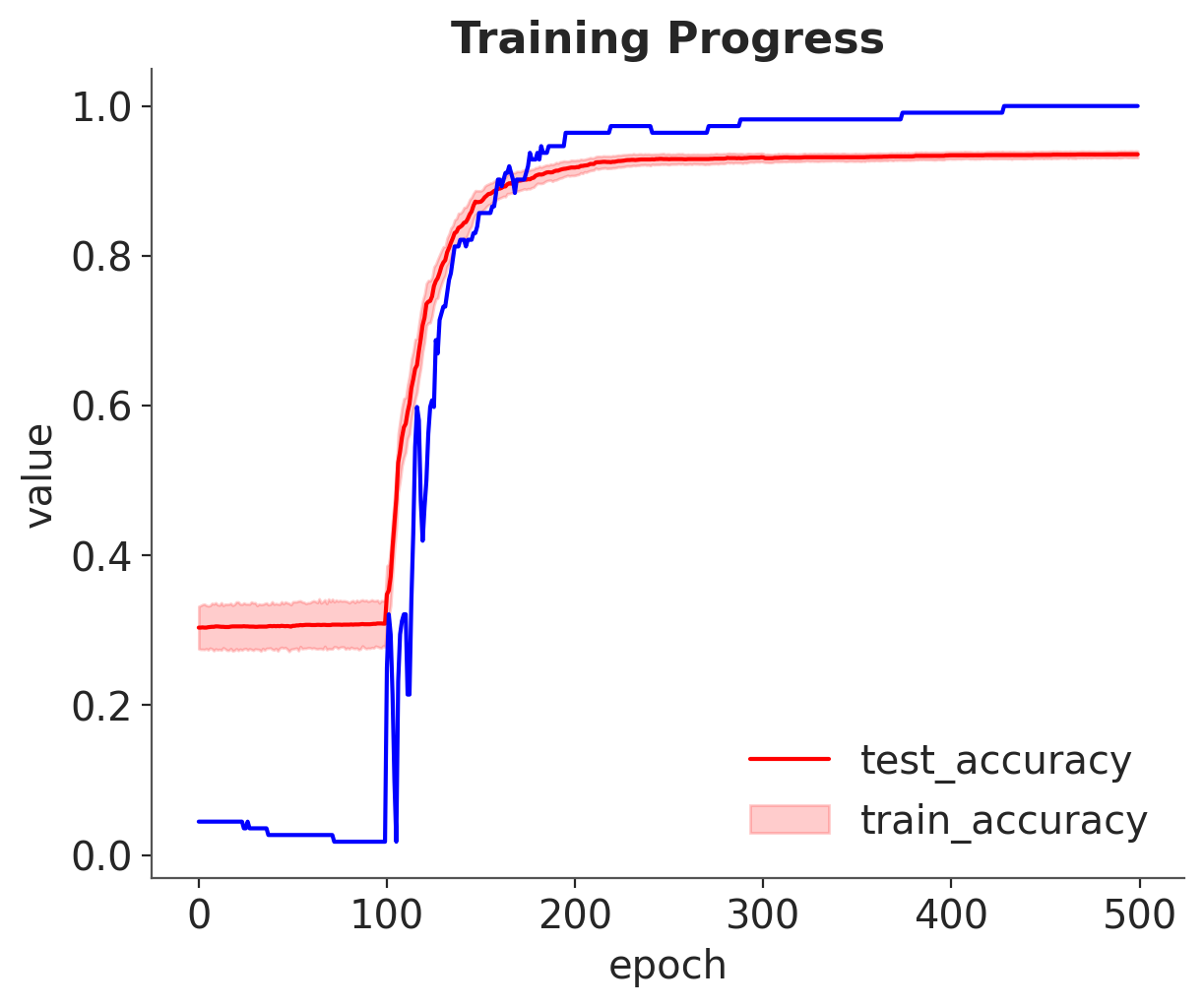
This is much better!

So, Tracker allows us to monitor our approximation and choose good training schedule.

Minibatches

When dealing with large datasets, using minibatch training can drastically speed up and improve approximation performance. Large datasets impose a hefty cost on the computation of gradients.

There is a nice API in PyMC to handle these cases, which is available through the pm.Minibatch class. The minibatch is just a highly specialized PyTensor tensor.

To demonstrate, let’s simulate a large quantity of data:

# Raw values
data = np.random.rand(40000, 100)
# Scaled values
data *= np.random.randint(1, 10, size=(100,))
# Shifted values
data += np.random.rand(100) * 10

For comparison, let’s fit a model without minibatch processing:

with pm.Model() as model:
    mu = pm.Flat("mu", shape=(100,))
    sd = pm.HalfNormal("sd", shape=(100,))
    lik = pm.Normal("lik", mu, sigma=sd, observed=data)

Just for fun, let’s create a custom special purpose callback to halt slow optimization. Here we define a callback that causes a hard stop when approximation runs too slowly:

def stop_after_10(approx, loss_history, i):
    if (i > 0) and (i % 10) == 0:
        raise StopIteration("I was slow, sorry")

with model:
    advifit = pm.fit(callbacks=[stop_after_10])

I was slow, sorry

Interrupted at 9 [0%]: Average Loss = 3.5125e+08

Inference is too slow, taking several seconds per iteration; fitting the approximation would have taken hours!

Now let’s use minibatches. At every iteration, we will draw 500 random values:

Remember to set total_size in observed

total_size is an important parameter that allows PyMC to infer the right way of rescaling densities. If it is not set, you are likely to get completely wrong results. For more information please refer to the comprehensive documentation of pm.Minibatch.

X = pm.Minibatch(data, batch_size=500)

with pm.Model() as model:
    mu = pm.Normal("mu", 0, sigma=1e5, shape=(100,))
    sd = pm.HalfNormal("sd", shape=(100,))
    likelihood = pm.Normal("likelihood", mu, sigma=sd, observed=X, total_size=data.shape[0])

with model:
    advifit = pm.fit()

Finished [100%]: Average Loss = 379.73

plt.plot(advifit.hist);

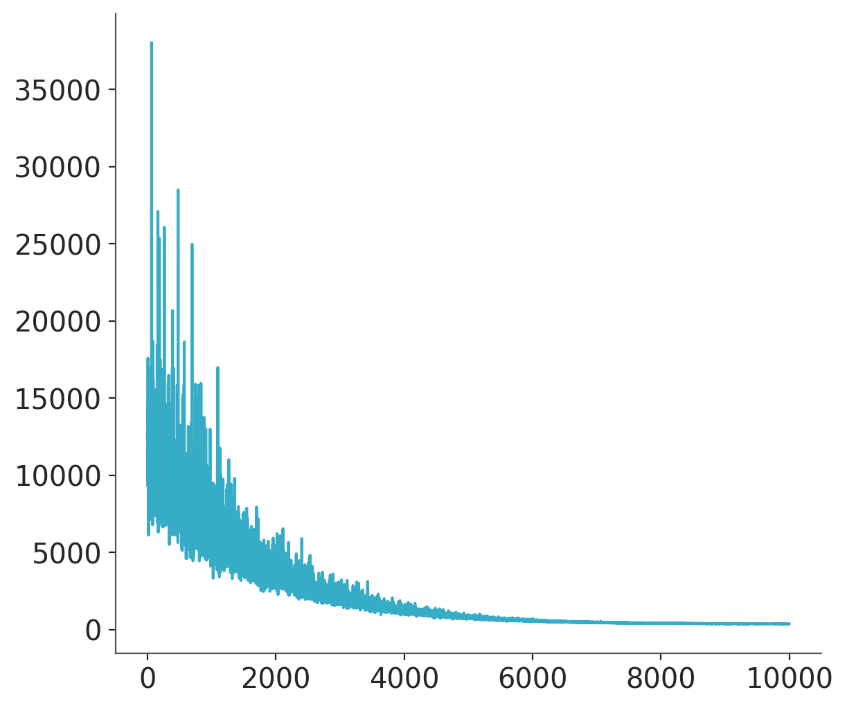
Minibatch inference is dramatically faster. Multidimensional minibatches may be needed for some corner cases where you do matrix factorization or model is very wide.

Here is the docstring for Minibatch to illustrate how it can be customized.

print(pm.Minibatch.__doc__)

Get random slices from variables from the leading dimension.

    Parameters
    ----------
    variable: TensorVariable
    variables: TensorVariable
    batch_size: int

    Examples
    --------
    >>> data1 = np.random.randn(100, 10)
    >>> data2 = np.random.randn(100, 20)
    >>> mdata1, mdata2 = Minibatch(data1, data2, batch_size=10)
    

Authors

• Authored by Maxim Kochurov

• Updated by Chris Fonnesbeck (pymc-examples#429)

Watermark

%load_ext watermark
%watermark -n -u -v -iv -w

Last updated: Mon, 25 May 2026

Python implementation: CPython
Python version       : 3.12.12
IPython version      : 9.13.0

arviz     : 1.1.0
matplotlib: 3.10.9
numpy     : 2.4.6
pandas    : 3.0.3
platform  : 1.0.8
pymc      : 6.0.1
pytensor  : 3.0.3
seaborn   : 0.13.2
sklearn   : 1.8.0

Watermark: 2.6.0

License notice

All the notebooks in this example gallery are provided under the MIT License which allows modification, and redistribution for any use provided the copyright and license notices are preserved.

Citing PyMC examples

To cite this notebook, use the DOI provided by Zenodo for the pymc-examples repository.

Important

Many notebooks are adapted from other sources: blogs, books… In such cases you should cite the original source as well.

Also remember to cite the relevant libraries used by your code.

Here is an citation template in bibtex:

@incollection{citekey,
  author    = "<notebook authors, see above>",
  title     = "<notebook title>",
  editor    = "PyMC Team",
  booktitle = "PyMC examples",
  doi       = "10.5281/zenodo.5654871"
}

which once rendered could look like: