Forecasting with Structural AR Timeseries#

Bayesian structural timeseries models are an interesting way to learn about the structure inherent in any observed timeseries data. It also gives us the ability to project forward the implied predictive distribution granting us another view on forecasting problems. We can treat the learned characteristics of the timeseries data observed to-date as informative about the structure of the unrealised future state of the same measure.

In this notebook we’ll see how to fit and predict a range of auto-regressive structural timeseries models and, importantly, how to predict future observations of the models.

import arviz as az
import numpy as np
import pandas as pd
import pymc as pm

from matplotlib import pyplot as plt

RANDOM_SEED = 8929
rng = np.random.default_rng(RANDOM_SEED)
az.style.use("arviz-darkgrid")

Generate Fake Autoregressive Data#

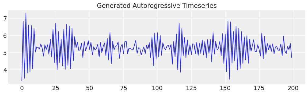
First we will generate a simple autoregressive timeseries. We will show how to specify a model to fit this data and then add a number of complexities to the data and show how they too can be captured with an autoregressive model and used to predict the shape of the future.

def simulate_ar(intercept, coef1, coef2, noise=0.3, *, warmup=10, steps=200):
    # We sample some extra warmup steps, to let the AR process stabilize
    draws = np.zeros(warmup + steps)
    # Initialize first draws at intercept
    draws[:2] = intercept
    for step in range(2, warmup + steps):
        draws[step] = (
            intercept
            + coef1 * draws[step - 1]
            + coef2 * draws[step - 2]
            + np.random.normal(0, noise)
        )
    # Discard the warmup draws
    return draws[warmup:]


# True parameters of the AR process
ar1_data = simulate_ar(10, -0.9, 0)

fig, ax = plt.subplots(figsize=(10, 3))
ax.set_title("Generated Autoregressive Timeseries", fontsize=15)
ax.plot(ar1_data);

../_images/a72e7a83bd44131c4c544f52c3de3fb4df7aaf7e9b41e35f5981c9868c69b765.png

Specifying the Model#

We’ll walk through the model step by step and then generalise the pattern into a function that can be used to take increasingly complex structural combinations of components.

## Set up a dictionary for the specification of our priors
## We set up the dictionary to specify size of the AR coefficients in
## case we want to vary the AR lags.
priors = {
    "coefs": {"mu": [10, 0.2], "sigma": [0.1, 0.1], "size": 2},
    "sigma": 8,
    "init": {"mu": 9, "sigma": 0.1, "size": 1},
}

## Initialise the model
with pm.Model() as AR:
    pass

## Define the time interval for fitting the data
t_data = list(range(len(ar1_data)))
## Add the time interval as a mutable coordinate to the model to allow for future predictions
AR.add_coord("obs_id", t_data, mutable=True)

with AR:
    ## Data containers to enable prediction
    t = pm.MutableData("t", t_data, dims="obs_id")
    y = pm.MutableData("y", ar1_data, dims="obs_id")

    # The first coefficient will be the constant term but we need to set priors for each coefficient in the AR process
    coefs = pm.Normal("coefs", priors["coefs"]["mu"], priors["coefs"]["sigma"])
    sigma = pm.HalfNormal("sigma", priors["sigma"])
    # We need one init variable for each lag, hence size is variable too
    init = pm.Normal.dist(
        priors["init"]["mu"], priors["init"]["sigma"], size=priors["init"]["size"]
    )
    # Steps of the AR model minus the lags required
    ar1 = pm.AR(
        "ar",
        coefs,
        sigma=sigma,
        init_dist=init,
        constant=True,
        steps=t.shape[0] - (priors["coefs"]["size"] - 1),
        dims="obs_id",
    )

    # The Likelihood
    outcome = pm.Normal("likelihood", mu=ar1, sigma=sigma, observed=y, dims="obs_id")
    ## Sampling
    idata_ar = pm.sample_prior_predictive()
    idata_ar.extend(pm.sample(2000, random_seed=100, target_accept=0.95))
    idata_ar.extend(pm.sample_posterior_predictive(idata_ar))

Sampling: [ar, coefs, likelihood, sigma]
Auto-assigning NUTS sampler...
Initializing NUTS using jitter+adapt_diag...
Multiprocess sampling (4 chains in 4 jobs)
NUTS: [coefs, sigma, ar]

100.00% [12000/12000 00:26<00:00 Sampling 4 chains, 0 divergences]

Sampling 4 chains for 1_000 tune and 2_000 draw iterations (4_000 + 8_000 draws total) took 46 seconds.
Sampling: [likelihood]

100.00% [8000/8000 00:00<00:00]

Lets check the model structure with plate notation and then examine the convergence diagnostics.

az.plot_trace(idata_ar, figsize=(10, 6), kind="rank_vlines");

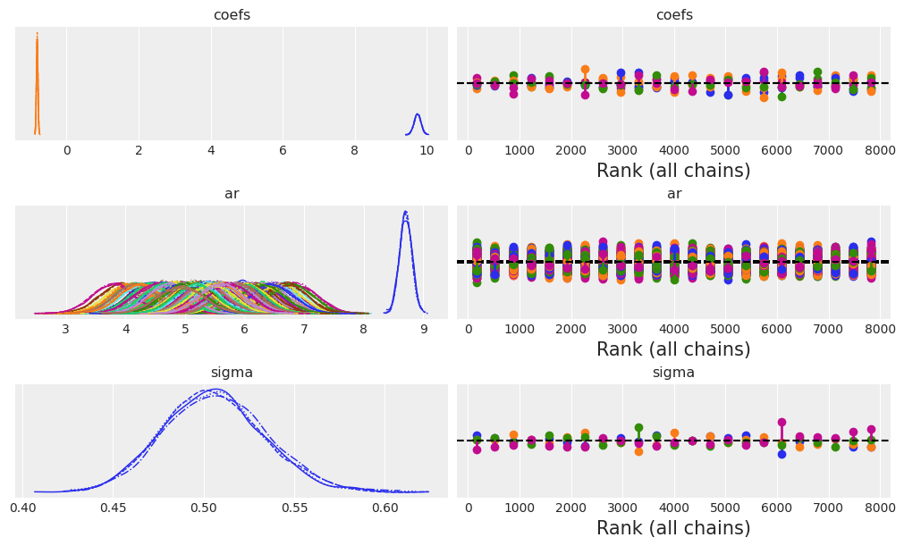
../_images/d89679b6818cb9e3a3ec9c556a88886cb17d4cd46eb9d20281216a1863a6d8f2.png

Next we’ll check the summary estimates for the to AR coefficients and the sigma term.

az.summary(idata_ar, var_names=["~ar"])

	mean	sd	hdi_3%	hdi_97%	mcse_mean	mcse_sd	ess_bulk	ess_tail	r_hat
coefs[0]	9.744	0.094	9.555	9.911	0.001	0.001	13107.0	6200.0	1.0
coefs[1]	-0.815	0.021	-0.854	-0.776	0.000	0.000	9141.0	5792.0	1.0
sigma	0.506	0.028	0.453	0.557	0.001	0.000	2965.0	5254.0	1.0

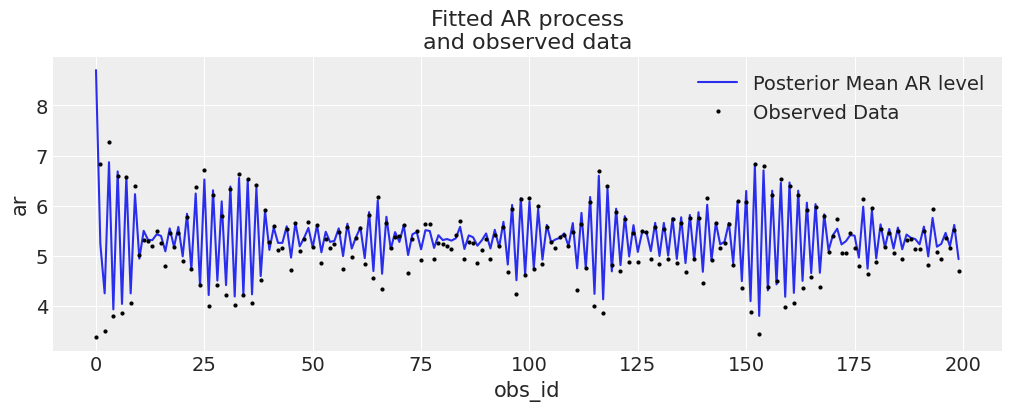
We can see here that the model fit has fairly correctly estimated the true parameters of the data generating process. We can also see this if we plot the posterior ar distribution against our observed data.

fig, ax = plt.subplots(figsize=(10, 4))
idata_ar.posterior.ar.mean(["chain", "draw"]).plot(ax=ax, label="Posterior Mean AR level")
ax.plot(ar1_data, "o", color="black", markersize=2, label="Observed Data")
ax.legend()
ax.set_title("Fitted AR process\nand observed data");

../_images/9bb5fa7766e0dfa6c0375e9c37f68c925411d36bec022d5264ca732b075e14bf.png

Inspecting model fit and forecast#

We can look at the standard posterior predictive fits but since our data is timeseries data we have to also look how draws from the posterior predictive distribution vary over time.

def plot_fits(idata_ar, idata_preds):
    palette = "plasma"
    cmap = plt.get_cmap(palette)
    percs = np.linspace(51, 99, 100)
    colors = (percs - np.min(percs)) / (np.max(percs) - np.min(percs))
    mosaic = """AABB
                CCCC"""
    fig, axs = plt.subplot_mosaic(mosaic, sharex=False, figsize=(20, 10))
    axs = [axs[k] for k in axs.keys()]
    for i, p in enumerate(percs[::-1]):
        upper = np.percentile(
            az.extract_dataset(idata_ar, group="prior_predictive", num_samples=1000)["likelihood"],
            p,
            axis=1,
        )
        lower = np.percentile(
            az.extract_dataset(idata_ar, group="prior_predictive", num_samples=1000)["likelihood"],
            100 - p,
            axis=1,
        )
        color_val = colors[i]
        axs[0].fill_between(
            x=idata_ar["constant_data"]["t"],
            y1=upper.flatten(),
            y2=lower.flatten(),
            color=cmap(color_val),
            alpha=0.1,
        )

    axs[0].plot(
        az.extract_dataset(idata_ar, group="prior_predictive", num_samples=1000)["likelihood"].mean(
            axis=1
        ),
        color="cyan",
        label="Prior Predicted Mean Realisation",
    )

    axs[0].scatter(
        x=idata_ar["constant_data"]["t"],
        y=idata_ar["constant_data"]["y"],
        color="k",
        label="Observed Data points",
    )
    axs[0].set_title("Prior Predictive Fit", fontsize=20)
    axs[0].legend()

    for i, p in enumerate(percs[::-1]):
        upper = np.percentile(
            az.extract_dataset(idata_preds, group="predictions", num_samples=1000)["likelihood"],
            p,
            axis=1,
        )
        lower = np.percentile(
            az.extract_dataset(idata_preds, group="predictions", num_samples=1000)["likelihood"],
            100 - p,
            axis=1,
        )
        color_val = colors[i]
        axs[2].fill_between(
            x=idata_preds["predictions_constant_data"]["t"],
            y1=upper.flatten(),
            y2=lower.flatten(),
            color=cmap(color_val),
            alpha=0.1,
        )

        upper = np.percentile(
            az.extract_dataset(idata_preds, group="predictions", num_samples=1000)["yhat_fut"],
            p,
            axis=1,
        )
        lower = np.percentile(
            az.extract_dataset(idata_preds, group="predictions", num_samples=1000)["yhat_fut"],
            100 - p,
            axis=1,
        )
        color_val = colors[i]
        axs[2].fill_between(
            x=idata_preds["predictions"].coords["obs_id_fut"].data,
            y1=upper.flatten(),
            y2=lower.flatten(),
            color=cmap(color_val),
            alpha=0.1,
        )

    axs[2].plot(
        az.extract_dataset(idata_preds, group="predictions", num_samples=1000)["likelihood"].mean(
            axis=1
        ),
        color="cyan",
    )
    idata_preds.predictions.yhat_fut.mean(["chain", "draw"]).plot(
        ax=axs[2], color="cyan", label="Predicted Mean Realisation"
    )
    axs[2].scatter(
        x=idata_ar["constant_data"]["t"],
        y=idata_ar["constant_data"]["y"],
        color="k",
        label="Observed Data",
    )
    axs[2].set_title("Posterior Predictions Plotted", fontsize=20)
    axs[2].axvline(np.max(idata_ar["constant_data"]["t"]), color="black")
    axs[2].legend()
    axs[2].set_xlabel("Time in Days")
    axs[0].set_xlabel("Time in Days")
    az.plot_ppc(idata_ar, ax=axs[1])


plot_fits(idata_ar, idata_preds)

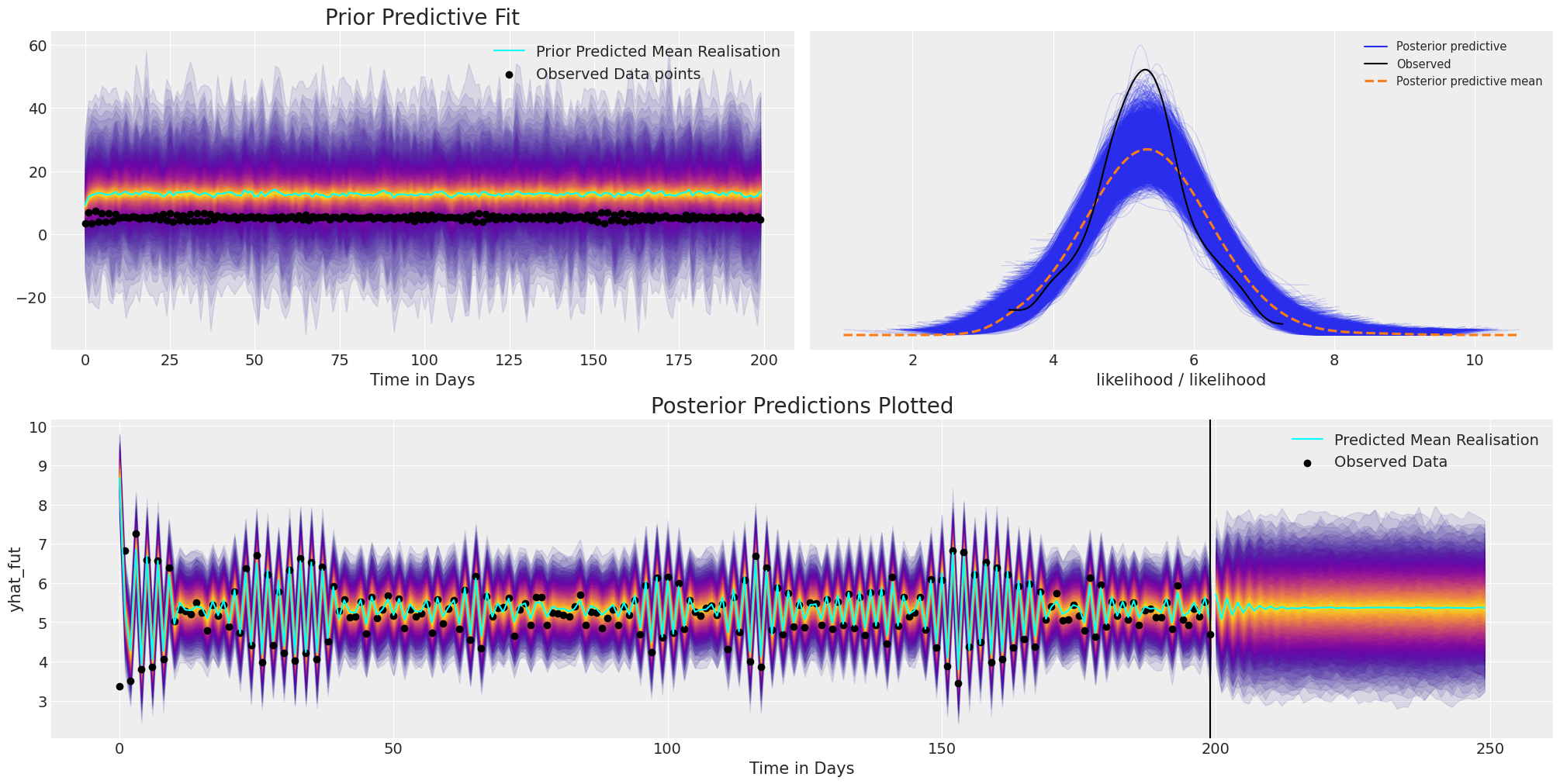
../_images/50c1547d7d5179e56668f96f85b4fa8923caf69edefeea7a5fcfed87168d99d5.png

Here we can see that although the model converged and ends up with a reasonable fit to the existing data, and a plausible projection for future values. However, we have set the prior specification very poorly in allowing an absurdly broad range of values due to the kind of compounding logic of the auto-regressive function. For this reason it’s very important to be able to inspect and tailor your model with prior predictive checks.

Secondly, the mean forecast fails to capture any long lasting structure, quickly dying down to a stable baseline. To account for these kind of short-lived forecasts, we can add more structure to our model, but first, let’s complicate the picture.

Complicating the Picture#

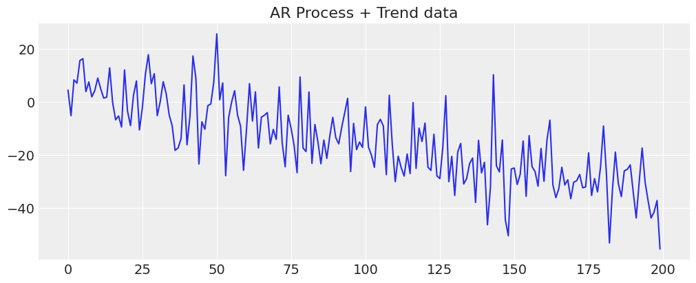
Often our data will involve more than one latent process, and might have more complex factors which drive the outcomes. To see one such complication let’s add a trend to our data. By adding more structure to our forecast we are telling our model that we expect certain patterns or trends to remain in the data out into the future. The choice of which structures to add are at the discretion of the creative modeller - here we’ll demonstrate some simple examples.

y_t = -0.3 + np.arange(200) * -0.2 + np.random.normal(0, 10, 200)
y_t = y_t + ar1_data

fig, ax = plt.subplots(figsize=(10, 4))
ax.plot(y_t)
ax.set_title("AR Process + Trend data");

../_images/60f92ba6eb44c8cdab53d78b81da6e84c3d3e8cc024556a1b6e60f5897c0ee3a.png

Wrapping our model into a function#

def make_latent_AR_model(ar_data, priors, prediction_steps=250, full_sample=True, samples=2000):
    with pm.Model() as AR:
        pass

    t_data = list(range(len(ar_data)))
    AR.add_coord("obs_id", t_data, mutable=True)

    with AR:
        ## Data containers to enable prediction
        t = pm.MutableData("t", t_data, dims="obs_id")
        y = pm.MutableData("y", ar_data, dims="obs_id")
        # The first coefficient will be the intercept term
        coefs = pm.Normal("coefs", priors["coefs"]["mu"], priors["coefs"]["sigma"])
        sigma = pm.HalfNormal("sigma", priors["sigma"])
        # We need one init variable for each lag, hence size is variable too
        init = pm.Normal.dist(
            priors["init"]["mu"], priors["init"]["sigma"], size=priors["init"]["size"]
        )
        # Steps of the AR model minus the lags required given specification
        ar1 = pm.AR(
            "ar",
            coefs,
            sigma=sigma,
            init_dist=init,
            constant=True,
            steps=t.shape[0] - (priors["coefs"]["size"] - 1),
            dims="obs_id",
        )

        # The Likelihood
        outcome = pm.Normal("likelihood", mu=ar1, sigma=sigma, observed=y, dims="obs_id")
        ## Sampling
        idata_ar = pm.sample_prior_predictive()
        if full_sample:
            idata_ar.extend(pm.sample(samples, random_seed=100, target_accept=0.95))
            idata_ar.extend(pm.sample_posterior_predictive(idata_ar))
        else:
            return idata_ar

    n = prediction_steps - ar_data.shape[0]

    with AR:
        AR.add_coords({"obs_id_fut_1": range(ar1_data.shape[0] - 1, 250, 1)})
        AR.add_coords({"obs_id_fut": range(ar1_data.shape[0], 250, 1)})
        # condition on the learned values of the AR process
        # initialise the future AR process precisely at the last observed value in the AR process
        # using the special feature of the dirac delta distribution to be 0 probability everywhere else.
        ar1_fut = pm.AR(
            "ar1_fut",
            init_dist=pm.DiracDelta.dist(ar1[..., -1]),
            rho=coefs,
            sigma=sigma,
            constant=True,
            dims="obs_id_fut_1",
        )
        yhat_fut = pm.Normal("yhat_fut", mu=ar1_fut[1:], sigma=sigma, dims="obs_id_fut")
        # use the updated values and predict outcomes and probabilities:
        idata_preds = pm.sample_posterior_predictive(
            idata_ar, var_names=["likelihood", "yhat_fut"], predictions=True, random_seed=100
        )

    return idata_ar, idata_preds, AR

Next we’ll cycle through a number of prior specifications to show how that impacts the prior predictive distribution i.e. the implied distribution of our outcome if we were to forward sample from the model specified by our priors.

priors_0 = {
    "coefs": {"mu": [-4, 0.2], "sigma": 0.1, "size": 2},
    "sigma": 8,
    "init": {"mu": 9, "sigma": 0.1, "size": 1},
}

priors_1 = {
    "coefs": {"mu": [-2, 0.2], "sigma": 0.1, "size": 2},
    "sigma": 12,
    "init": {"mu": 8, "sigma": 0.1, "size": 1},
}

priors_2 = {
    "coefs": {"mu": [0, 0.2], "sigma": 0.1, "size": 2},
    "sigma": 15,
    "init": {"mu": 8, "sigma": 0.1, "size": 1},
}

models = {}
for i, p in enumerate([priors_0, priors_1, priors_2]):
    models[i] = {}
    idata = make_latent_AR_model(y_t, p, full_sample=False)
    models[i]["idata"] = idata

Sampling: [ar, coefs, likelihood, sigma]
Sampling: [ar, coefs, likelihood, sigma]
Sampling: [ar, coefs, likelihood, sigma]

fig, axs = plt.subplots(1, 3, figsize=(10, 4), sharey=True)
axs = axs.flatten()
for i, p in zip(range(3), [priors_0, priors_1, priors_2]):
    axs[i].plot(
        az.extract_dataset(models[i]["idata"], group="prior_predictive", num_samples=100)[
            "likelihood"
        ],
        color="blue",
        alpha=0.1,
    )
    axs[i].plot(y_t, "o", color="black", markersize=2)
    axs[i].set_title(
        "$y_{t+1}$" + f'= N({p["coefs"]["mu"][0]} + {p["coefs"]["mu"][1]}y$_t$, {p["sigma"]})'
    )
plt.suptitle("Prior Predictive Specifications", fontsize=20);

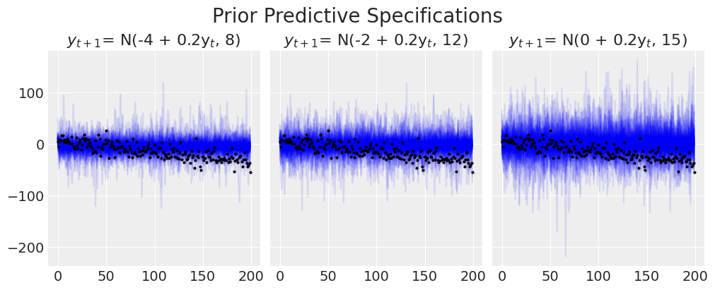
../_images/382fa52b8854574ad31a5a7213a0d0859dbd3a682d00e4da19051733e948e75b.png

We can see the manner in which the model struggles to capture the trend line. Increasing the variability of the model will never capture the directional pattern we know to be in the data.

priors_0 = {
    "coefs": {"mu": [-4, 0.2], "sigma": [0.5, 0.03], "size": 2},
    "sigma": 8,
    "init": {"mu": -4, "sigma": 0.1, "size": 1},
}

idata_no_trend, preds_no_trend, model = make_latent_AR_model(y_t, priors_0)

Sampling: [ar, coefs, likelihood, sigma]
Auto-assigning NUTS sampler...
Initializing NUTS using jitter+adapt_diag...
Multiprocess sampling (4 chains in 4 jobs)
NUTS: [coefs, sigma, ar]

100.00% [12000/12000 00:22<00:00 Sampling 4 chains, 0 divergences]

Sampling 4 chains for 1_000 tune and 2_000 draw iterations (4_000 + 8_000 draws total) took 49 seconds.
Sampling: [likelihood]

100.00% [8000/8000 00:00<00:00]

Sampling: [ar1_fut, likelihood, yhat_fut]

100.00% [8000/8000 00:29<00:00]

plot_fits(idata_no_trend, preds_no_trend)

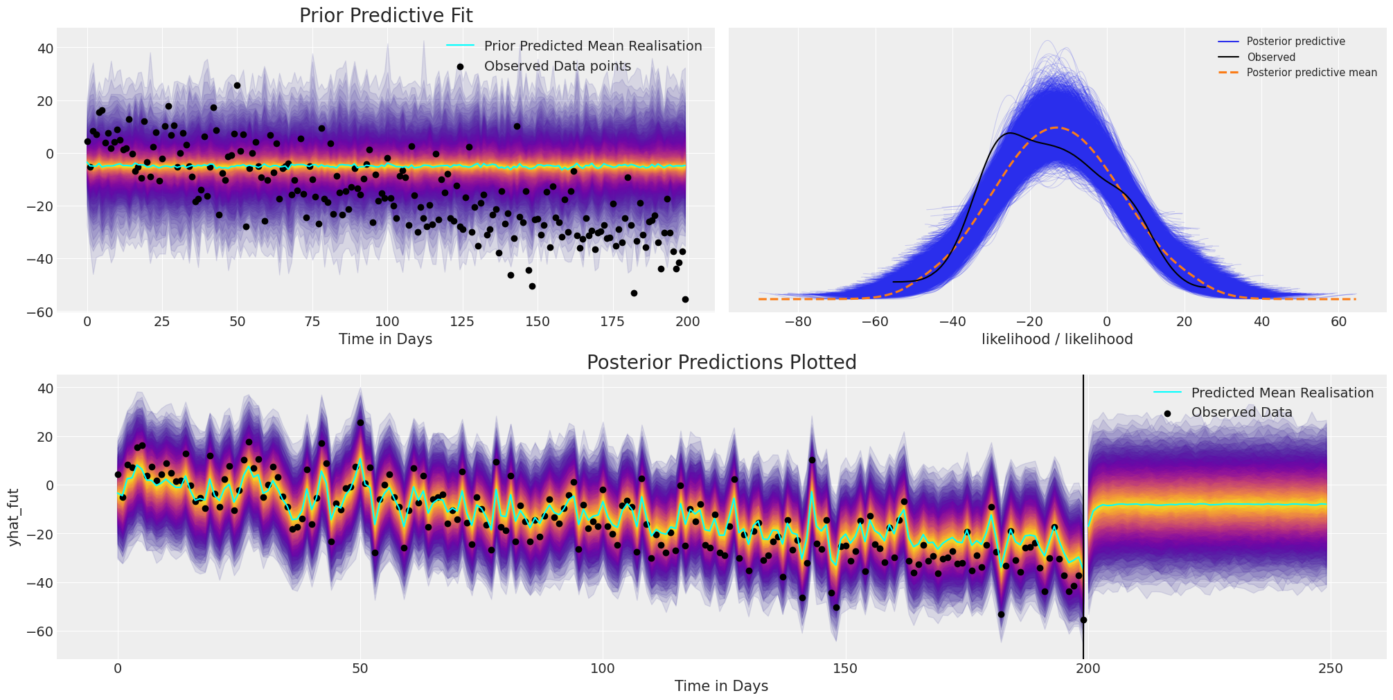
../_images/964c239d241b2d5fe552c598f317302019331701e8d254575779447c685e984a.png

Forecasting with this model is somewhat hopeless because, while the model fit adjusts well with observed data, but it completely fails to capture the structural trend in the data. So without some structural constraint when we seek to make predictions with this simple AR model, it reverts to the mean level forecast very quickly.

Specifying a Trend Model#

We will define a model to account for the trend in our data and combine this trend in an additive model with the autoregressive components. Again the model is much as before, but now we add additional latent features. These are to be combined in a simple additive combination but we can be more creative here if it would suit our model.

def make_latent_AR_trend_model(
    ar_data, priors, prediction_steps=250, full_sample=True, samples=2000
):
    with pm.Model() as AR:
        pass

    t_data = list(range(len(ar_data)))
    AR.add_coord("obs_id", t_data, mutable=True)

    with AR:
        ## Data containers to enable prediction
        t = pm.MutableData("t", t_data, dims="obs_id")
        y = pm.MutableData("y", ar_data, dims="obs_id")
        # The first coefficient will be the intercept term
        coefs = pm.Normal("coefs", priors["coefs"]["mu"], priors["coefs"]["sigma"])
        sigma = pm.HalfNormal("sigma", priors["sigma"])
        # We need one init variable for each lag, hence size is variable too
        init = pm.Normal.dist(
            priors["init"]["mu"], priors["init"]["sigma"], size=priors["init"]["size"]
        )
        # Steps of the AR model minus the lags required given specification
        ar1 = pm.AR(
            "ar",
            coefs,
            sigma=sigma,
            init_dist=init,
            constant=True,
            steps=t.shape[0] - (priors["coefs"]["size"] - 1),
            dims="obs_id",
        )

        ## Priors for the linear trend component
        alpha = pm.Normal("alpha", priors["alpha"]["mu"], priors["alpha"]["sigma"])
        beta = pm.Normal("beta", priors["beta"]["mu"], priors["beta"]["sigma"])
        trend = pm.Deterministic("trend", alpha + beta * t, dims="obs_id")

        mu = ar1 + trend

        # The Likelihood
        outcome = pm.Normal("likelihood", mu=mu, sigma=sigma, observed=y, dims="obs_id")
        ## Sampling
        idata_ar = pm.sample_prior_predictive()
        if full_sample:
            idata_ar.extend(pm.sample(samples, random_seed=100, target_accept=0.95))
            idata_ar.extend(pm.sample_posterior_predictive(idata_ar))
        else:
            return idata_ar

    n = prediction_steps - ar_data.shape[0]

    with AR:
        AR.add_coords({"obs_id_fut_1": range(ar1_data.shape[0] - 1, prediction_steps, 1)})
        AR.add_coords({"obs_id_fut": range(ar1_data.shape[0], prediction_steps, 1)})
        t_fut = pm.MutableData("t_fut", list(range(ar1_data.shape[0], prediction_steps, 1)))
        # condition on the learned values of the AR process
        # initialise the future AR process precisely at the last observed value in the AR process
        # using the special feature of the dirac delta distribution to be 0 probability everywhere else.
        ar1_fut = pm.AR(
            "ar1_fut",
            init_dist=pm.DiracDelta.dist(ar1[..., -1]),
            rho=coefs,
            sigma=sigma,
            constant=True,
            dims="obs_id_fut_1",
        )
        trend = pm.Deterministic("trend_fut", alpha + beta * t_fut, dims="obs_id_fut")
        mu = ar1_fut[1:] + trend

        yhat_fut = pm.Normal("yhat_fut", mu=mu, sigma=sigma, dims="obs_id_fut")
        # use the updated values and predict outcomes and probabilities:
        idata_preds = pm.sample_posterior_predictive(
            idata_ar, var_names=["likelihood", "yhat_fut"], predictions=True, random_seed=100
        )

    return idata_ar, idata_preds, AR

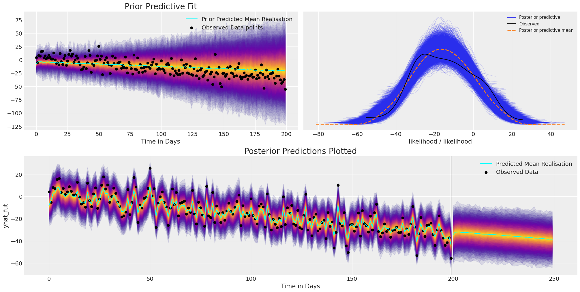
We will fit this model by specifying priors on the negative trend and the range of the standard deviation to respect the direction of the data drift.

priors_0 = {
    "coefs": {"mu": [0.2, 0.2], "sigma": [0.5, 0.03], "size": 2},
    "alpha": {"mu": -4, "sigma": 0.1},
    "beta": {"mu": -0.1, "sigma": 0.2},
    "sigma": 8,
    "init": {"mu": -4, "sigma": 0.1, "size": 1},
}


idata_trend, preds_trend, model = make_latent_AR_trend_model(y_t, priors_0, full_sample=True)

Sampling: [alpha, ar, beta, coefs, likelihood, sigma]
Auto-assigning NUTS sampler...
Initializing NUTS using jitter+adapt_diag...
Multiprocess sampling (4 chains in 4 jobs)
NUTS: [coefs, sigma, ar, alpha, beta]

100.00% [12000/12000 00:33<00:00 Sampling 4 chains, 0 divergences]

Sampling 4 chains for 1_000 tune and 2_000 draw iterations (4_000 + 8_000 draws total) took 57 seconds.
Sampling: [likelihood]

100.00% [8000/8000 00:00<00:00]

Sampling: [ar1_fut, likelihood, yhat_fut]

100.00% [8000/8000 00:30<00:00]

pm.model_to_graphviz(model)

../_images/734d82652185212052440dcf2a189d4862d7b6bf22f4bd4e1f64ff5d9032a80a.svg

We can see the structure more clearly with the plate notation, and this additional structure has helped to appropriately fit the directional trend of the timeseries data.

plot_fits(idata_trend, preds_trend);

../_images/722bf61555339ad1f1329e95ebd305407a4d42c1516adc7d792ae0757a5c1d1e.png

az.summary(idata_trend, var_names=["coefs", "sigma", "alpha", "beta"])

	mean	sd	hdi_3%	hdi_97%	mcse_mean	mcse_sd	ess_bulk	ess_tail	r_hat
coefs[0]	1.086	0.475	0.220	2.006	0.010	0.007	2482.0	4278.0	1.0
coefs[1]	0.210	0.029	0.156	0.264	0.000	0.000	7296.0	5931.0	1.0
sigma	7.557	0.389	6.841	8.284	0.007	0.005	3332.0	4817.0	1.0
alpha	-3.969	0.099	-4.171	-3.794	0.001	0.001	9220.0	5606.0	1.0
beta	-0.145	0.009	-0.161	-0.128	0.000	0.000	1785.0	3995.0	1.0

Complicating the picture further#

Next we’ll add a seasonal component to our data and see how we can recover this aspect of the data with a bayesian structural timeseries model. Again, this is is because in reality our data is often the result of multiple converging influences. These influences can be capture in an additive bayesian structural model where our inferential model ensures that we allocate appropriate weight to each of the components.

t_data = list(range(200))
n_order = 10
periods = np.array(t_data) / 7

fourier_features = pd.DataFrame(
    {
        f"{func}_order_{order}": getattr(np, func)(2 * np.pi * periods * order)
        for order in range(1, n_order + 1)
        for func in ("sin", "cos")
    }
)

y_t_s = y_t + 20 * fourier_features["sin_order_1"]

fig, ax = plt.subplots(figsize=(10, 4))
ax.plot(y_t_s)
ax.set_title("AR + Trend + Seasonality");

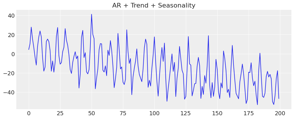
../_images/285e345411293af1986d5240b1c81a77d7681751d8dda5c72f03705d6f760f51.png

The key to fitting this model is to understand that we’re now passing in synthetic fourier features to help account for seasonality effects. This works because (roughly speaking) we’re trying to fit a complex oscillating phenomena using a weighted combination of sine and cosine waves. So we add these sine waves and consine waves like we would add any other feature variables in a regression model.

However, since we’re using this weighted sum to fit the observed data, the model now expects a linear combination of those synthetic features also in the prediction step. As such we need to be able to supply those features even out into the future. This fact remains key for any other type of predictive feature we might want to add e.g. day of the week, holiday dummy variable or any other. If a feature is required to fit the observed data the feature must be available in the prediction step too.

Specifying the Trend + Seasonal Model#

def make_latent_AR_trend_seasonal_model(
    ar_data, ff, priors, prediction_steps=250, full_sample=True, samples=2000
):
    with pm.Model() as AR:
        pass

    ff = ff.to_numpy().T
    t_data = list(range(len(ar_data)))
    AR.add_coord("obs_id", t_data, mutable=True)
    ## The fourier features must be mutable to allow for addition fourier features to be
    ## passed in the prediction step.
    AR.add_coord("fourier_features", np.arange(len(ff)), mutable=True)

    with AR:
        ## Data containers to enable prediction
        t = pm.MutableData("t", t_data, dims="obs_id")
        y = pm.MutableData("y", ar_data, dims="obs_id")
        # The first coefficient will be the intercept term
        coefs = pm.Normal("coefs", priors["coefs"]["mu"], priors["coefs"]["sigma"])
        sigma = pm.HalfNormal("sigma", priors["sigma"])
        # We need one init variable for each lag, hence size is variable too
        init = pm.Normal.dist(
            priors["init"]["mu"], priors["init"]["sigma"], size=priors["init"]["size"]
        )
        # Steps of the AR model minus the lags required given specification
        ar1 = pm.AR(
            "ar",
            coefs,
            sigma=sigma,
            init_dist=init,
            constant=True,
            steps=t.shape[0] - (priors["coefs"]["size"] - 1),
            dims="obs_id",
        )

        ## Priors for the linear trend component
        alpha = pm.Normal("alpha", priors["alpha"]["mu"], priors["alpha"]["sigma"])
        beta = pm.Normal("beta", priors["beta"]["mu"], priors["beta"]["sigma"])
        trend = pm.Deterministic("trend", alpha + beta * t, dims="obs_id")

        ## Priors for seasonality
        beta_fourier = pm.Normal(
            "beta_fourier",
            mu=priors["beta_fourier"]["mu"],
            sigma=priors["beta_fourier"]["sigma"],
            dims="fourier_features",
        )
        fourier_terms = pm.MutableData("fourier_terms", ff)
        seasonality = pm.Deterministic(
            "seasonality", pm.math.dot(beta_fourier, fourier_terms), dims="obs_id"
        )

        mu = ar1 + trend + seasonality

        # The Likelihood
        outcome = pm.Normal("likelihood", mu=mu, sigma=sigma, observed=y, dims="obs_id")
        ## Sampling
        idata_ar = pm.sample_prior_predictive()
        if full_sample:
            idata_ar.extend(pm.sample(samples, random_seed=100, target_accept=0.95))
            idata_ar.extend(pm.sample_posterior_predictive(idata_ar))
        else:
            return idata_ar

    n = prediction_steps - ar_data.shape[0]
    n_order = 10
    periods = (ar_data.shape[0] + np.arange(n)) / 7

    fourier_features_new = pd.DataFrame(
        {
            f"{func}_order_{order}": getattr(np, func)(2 * np.pi * periods * order)
            for order in range(1, n_order + 1)
            for func in ("sin", "cos")
        }
    )

    with AR:
        AR.add_coords({"obs_id_fut_1": range(ar1_data.shape[0] - 1, prediction_steps, 1)})
        AR.add_coords({"obs_id_fut": range(ar1_data.shape[0], prediction_steps, 1)})
        t_fut = pm.MutableData(
            "t_fut", list(range(ar1_data.shape[0], prediction_steps, 1)), dims="obs_id_fut"
        )
        ff_fut = pm.MutableData("ff_fut", fourier_features_new.to_numpy().T)
        # condition on the learned values of the AR process
        # initialise the future AR process precisely at the last observed value in the AR process
        # using the special feature of the dirac delta distribution to be 0 probability everywhere else.
        ar1_fut = pm.AR(
            "ar1_fut",
            init_dist=pm.DiracDelta.dist(ar1[..., -1]),
            rho=coefs,
            sigma=sigma,
            constant=True,
            dims="obs_id_fut_1",
        )
        trend = pm.Deterministic("trend_fut", alpha + beta * t_fut, dims="obs_id_fut")
        seasonality = pm.Deterministic(
            "seasonality_fut", pm.math.dot(beta_fourier, ff_fut), dims="obs_id_fut"
        )
        mu = ar1_fut[1:] + trend + seasonality

        yhat_fut = pm.Normal("yhat_fut", mu=mu, sigma=sigma, dims="obs_id_fut")
        # use the updated values and predict outcomes and probabilities:
        idata_preds = pm.sample_posterior_predictive(
            idata_ar, var_names=["likelihood", "yhat_fut"], predictions=True, random_seed=743
        )

    return idata_ar, idata_preds, AR

priors_0 = {
    "coefs": {"mu": [0.2, 0.2], "sigma": [0.5, 0.03], "size": 2},
    "alpha": {"mu": -4, "sigma": 0.1},
    "beta": {"mu": -0.1, "sigma": 0.2},
    "beta_fourier": {"mu": 0, "sigma": 2},
    "sigma": 8,
    "init": {"mu": -4, "sigma": 0.1, "size": 1},
}


idata_t_s, preds_t_s, model = make_latent_AR_trend_seasonal_model(y_t_s, fourier_features, priors_0)

Sampling: [alpha, ar, beta, beta_fourier, coefs, likelihood, sigma]
Auto-assigning NUTS sampler...
Initializing NUTS using jitter+adapt_diag...
Multiprocess sampling (4 chains in 4 jobs)
NUTS: [coefs, sigma, ar, alpha, beta, beta_fourier]

100.00% [12000/12000 00:43<00:00 Sampling 4 chains, 0 divergences]

Sampling 4 chains for 1_000 tune and 2_000 draw iterations (4_000 + 8_000 draws total) took 70 seconds.
Sampling: [likelihood]

100.00% [8000/8000 00:01<00:00]

Sampling: [ar1_fut, likelihood, yhat_fut]

100.00% [8000/8000 00:31<00:00]

pm.model_to_graphviz(model)

../_images/b613ba6fad8c0d454e11cfaf3d67cf78bac628659453ff51f7c3361e710660e8.svg

az.summary(idata_t_s, var_names=["alpha", "beta", "coefs", "beta_fourier"])

	mean	sd	hdi_3%	hdi_97%	mcse_mean	mcse_sd	ess_bulk	ess_tail	r_hat
alpha	-3.986	0.099	-4.172	-3.797	0.001	0.001	13106.0	6145.0	1.0
beta	-0.182	0.012	-0.204	-0.159	0.000	0.000	3522.0	5420.0	1.0
coefs[0]	0.595	0.484	-0.287	1.536	0.009	0.006	3177.0	5203.0	1.0
coefs[1]	0.195	0.029	0.137	0.246	0.000	0.000	11284.0	6668.0	1.0
beta_fourier[0]	5.700	1.681	2.558	8.785	0.018	0.013	8413.0	5505.0	1.0
beta_fourier[1]	0.275	1.647	-2.913	3.280	0.018	0.018	8501.0	5712.0	1.0
beta_fourier[2]	0.188	1.641	-2.862	3.241	0.017	0.017	9114.0	5857.0	1.0
beta_fourier[3]	-0.066	1.669	-3.209	3.026	0.018	0.018	8683.0	6748.0	1.0
beta_fourier[4]	0.172	1.667	-2.771	3.382	0.017	0.018	9684.0	6683.0	1.0
beta_fourier[5]	-0.143	1.668	-3.285	2.910	0.017	0.018	9728.0	5846.0	1.0
beta_fourier[6]	-0.176	1.624	-3.215	2.860	0.017	0.018	9020.0	5924.0	1.0
beta_fourier[7]	-0.151	1.672	-3.222	3.015	0.017	0.018	9259.0	6636.0	1.0
beta_fourier[8]	-0.174	1.659	-3.277	2.944	0.017	0.018	9347.0	6390.0	1.0
beta_fourier[9]	-0.021	1.637	-3.198	2.878	0.018	0.017	8138.0	6374.0	1.0
beta_fourier[10]	-5.691	1.683	-8.789	-2.487	0.018	0.013	8219.0	6287.0	1.0
beta_fourier[11]	0.298	1.652	-2.769	3.415	0.018	0.018	8453.0	5843.0	1.0
beta_fourier[12]	0.016	2.041	-3.673	3.914	0.016	0.026	15708.0	5857.0	1.0
beta_fourier[13]	5.603	1.333	3.018	7.990	0.023	0.016	3460.0	5277.0	1.0
beta_fourier[14]	5.691	1.650	2.570	8.754	0.018	0.013	8261.0	6341.0	1.0
beta_fourier[15]	0.289	1.634	-2.897	3.245	0.018	0.018	8464.0	6278.0	1.0
beta_fourier[16]	0.214	1.654	-2.989	3.200	0.017	0.017	9169.0	6719.0	1.0
beta_fourier[17]	-0.031	1.663	-3.224	2.996	0.018	0.019	8464.0	5444.0	1.0
beta_fourier[18]	0.177	1.683	-2.978	3.316	0.018	0.020	9126.0	5907.0	1.0
beta_fourier[19]	-0.146	1.669	-3.339	2.925	0.018	0.019	8771.0	6316.0	1.0

plot_fits(idata_t_s, preds_t_s)

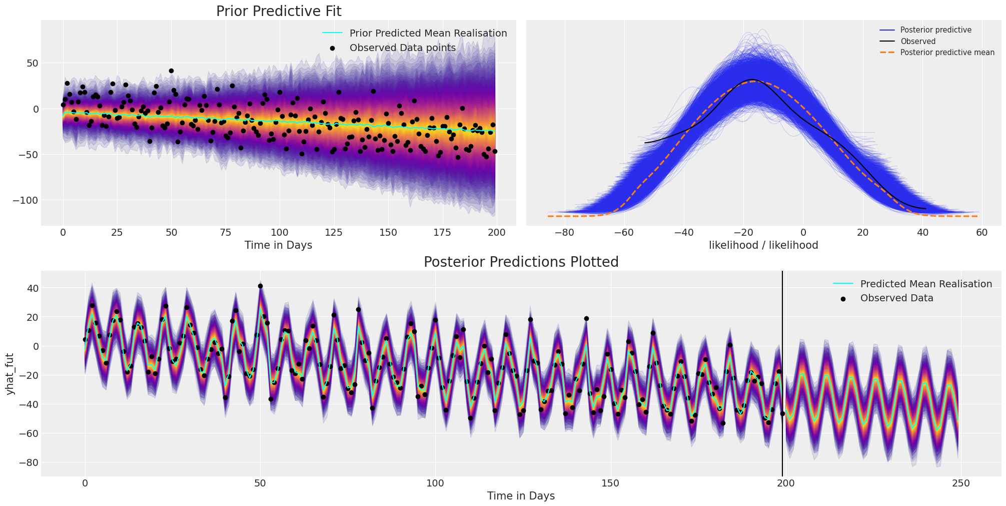
../_images/086ce40fad0e3bc0c9c718da0dfdb5a574c84aab65e5f6143f71fc0a52a227c7.png

We can see here how the model fit again recovers the broad structure and trend of the data, but in addition we have captured the oscillation of the seasonal effect and projected that into the future.

Closing Remarks#

The strength of a Bayesian model is largely the flexibility it offers for each modelling task. Hopefully this notebook gives a flavour of the variety of combinations worth considering when building a model to suit your use-case. We’ve seen how the Bayesian structural timeseries approach to forecasting can reveal the structure underlying our data, and be used to project that structure forward in time. We’ve seen how to encode different assumptions in the data generating model and calibrate our models against the observed data with posterior predictive checks.

Notably in the case of Auto-regressive modelling we’ve explicitly relied on the learned posterior distribution of the structural components. In this aspect we think the above is a kind of pure (neatly contained) example of Bayesian learning.

Authors#

Adapted from Nathaniel Forde’s Examined Algorithms Blog by Nathaniel Forde in Oct 2022.

Watermark#

%load_ext watermark
%watermark -n -u -v -iv -w -p pytensor,aeppl,xarray

Last updated: Wed Nov 09 2022

Python implementation: CPython
Python version       : 3.9.0
IPython version      : 8.4.0

pytensor: 2.8.7
aeppl : 0.0.38
xarray: 2022.10.0

arviz     : 0.12.1
pymc      : 4.2.2
numpy     : 1.23.4
pandas    : 1.5.1
sys       : 3.9.0 (default, Nov 15 2020, 06:25:35) 
[Clang 10.0.0 ]
matplotlib: 3.6.1

Watermark: 2.3.1

License notice#

All the notebooks in this example gallery are provided under the MIT License which allows modification, and redistribution for any use provided the copyright and license notices are preserved.

Citing PyMC examples#

To cite this notebook, use the DOI provided by Zenodo for the pymc-examples repository.

Important

Many notebooks are adapted from other sources: blogs, books… In such cases you should cite the original source as well.

Also remember to cite the relevant libraries used by your code.

Here is an citation template in bibtex:

@incollection{citekey,
  author    = "<notebook authors, see above>",
  title     = "<notebook title>",
  editor    = "PyMC Team",
  booktitle = "PyMC examples",
  doi       = "10.5281/zenodo.5654871"
}

which once rendered could look like:

Categories

Tags

Forecasting with Structural AR Timeseries#

Generate Fake Autoregressive Data#

Specifying the Model#

Prediction Step#

Inspecting model fit and forecast#

Complicating the Picture#

Wrapping our model into a function#

Specifying a Trend Model#

Complicating the picture further#

Specifying the Trend + Seasonal Model#

Closing Remarks#

Authors#

Watermark#

License notice#

Citing PyMC examples#