Air passengers - Prophet-like model

We’re going to look at the “air passengers” dataset, which tracks the monthly totals of a US airline passengers from 1949 to 1960. We could fit this using the Prophet model [Taylor and Letham, 2018] (indeed, this dataset is one of the examples they provide in their documentation), but instead we’ll make our own Prophet-like model in PyMC3. This will make it a lot easier to inspect the model’s components and to do prior predictive checks (an integral component of the Bayesian workflow [Gelman et al., 2020]).

import arviz as az
import matplotlib.dates as mdates
import matplotlib.pyplot as plt
import numpy as np
import pandas as pd
import pymc as pm

RANDOM_SEED = 8927
rng = np.random.default_rng(RANDOM_SEED)
az.style.use("arviz-darkgrid")
%config InlineBackend.figure_format = 'retina'

# get data
try:
    df = pd.read_csv("../data/AirPassengers.csv", parse_dates=["Month"])
except FileNotFoundError:
    df = pd.read_csv(pm.get_data("AirPassengers.csv"), parse_dates=["Month"])

Before we begin: visualise the data

df.plot.scatter(x="Month", y="#Passengers", color="k");

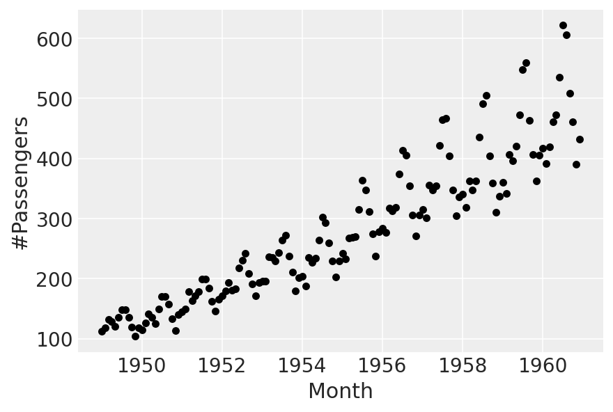
There’s an increasing trend, with multiplicative seasonality. We’ll fit a linear trend, and “borrow” the multiplicative seasonality part of it from Prophet.

Part 0: scale the data

First, we’ll scale time to be between 0 and 1:

t = (df["Month"] - pd.Timestamp("1900-01-01")).dt.days.to_numpy()
t_min = np.min(t)
t_max = np.max(t)
t = (t - t_min) / (t_max - t_min)

Next, for the target variable, we divide by the maximum. We do this, rather than standardising, so that the sign of the observations in unchanged - this will be necessary for the seasonality component to work properly later on.

y = df["#Passengers"].to_numpy()
y_max = np.max(y)
y = y / y_max

Part 1: linear trend

The model we’ll fit, for now, will just be

\[\text{Passengers} \sim \alpha + \beta\ \text{time}\]

First, let’s try using the default priors set by prophet, and we’ll do a prior predictive check:

with pm.Model(check_bounds=False) as linear:
    α = pm.Normal("α", mu=0, sigma=5)
    β = pm.Normal("β", mu=0, sigma=5)
    σ = pm.HalfNormal("σ", sigma=5)
    trend = pm.Deterministic("trend", α + β * t)
    pm.Normal("likelihood", mu=trend, sigma=σ, observed=y)

    linear_prior = pm.sample_prior_predictive()

fig, ax = plt.subplots(nrows=2, ncols=1, sharex=True)
ax[0].plot(
    df["Month"],
    az.extract_dataset(linear_prior, group="prior_predictive", num_samples=100)["likelihood"]
    * y_max,
    color="blue",
    alpha=0.05,
)
df.plot.scatter(x="Month", y="#Passengers", color="k", ax=ax[0])
ax[0].set_title("Prior predictive")
ax[1].plot(
    df["Month"],
    az.extract_dataset(linear_prior, group="prior", num_samples=100)["trend"] * y_max,
    color="blue",
    alpha=0.05,
)
df.plot.scatter(x="Month", y="#Passengers", color="k", ax=ax[1])
ax[1].set_title("Prior trend lines");

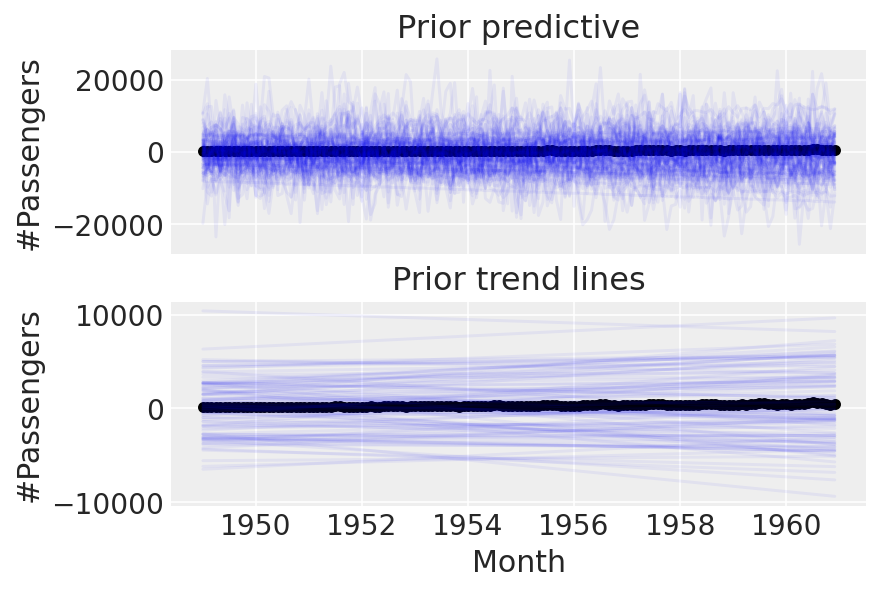
We can do better than this. These priors are evidently too wide, as we end up with implausibly many passengers. Let’s try setting tighter priors.

with pm.Model(check_bounds=False) as linear:
    α = pm.Normal("α", mu=0, sigma=0.5)
    β = pm.Normal("β", mu=0, sigma=0.5)
    σ = pm.HalfNormal("σ", sigma=0.1)
    trend = pm.Deterministic("trend", α + β * t)
    pm.Normal("likelihood", mu=trend, sigma=σ, observed=y)

    linear_prior = pm.sample_prior_predictive(samples=100)

fig, ax = plt.subplots(nrows=2, ncols=1, sharex=True)
ax[0].plot(
    df["Month"],
    az.extract_dataset(linear_prior, group="prior_predictive", num_samples=100)["likelihood"]
    * y_max,
    color="blue",
    alpha=0.05,
)
df.plot.scatter(x="Month", y="#Passengers", color="k", ax=ax[0])
ax[0].set_title("Prior predictive")
ax[1].plot(
    df["Month"],
    az.extract_dataset(linear_prior, group="prior", num_samples=100)["trend"] * y_max,
    color="blue",
    alpha=0.05,
)
df.plot.scatter(x="Month", y="#Passengers", color="k", ax=ax[1])
ax[1].set_title("Prior trend lines");

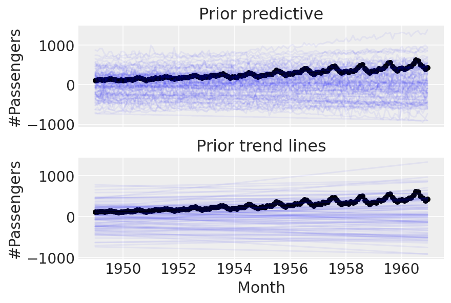
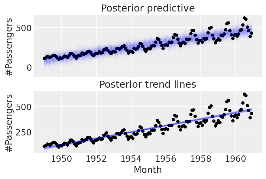
Cool. Before going on to anything more complicated, let’s try conditioning on the data and doing a posterior predictive check:

with linear:
    linear_trace = pm.sample(return_inferencedata=True)
    linear_prior = pm.sample_posterior_predictive(trace=linear_trace)

fig, ax = plt.subplots(nrows=2, ncols=1, sharex=True)
ax[0].plot(
    df["Month"],
    az.extract_dataset(linear_prior, group="posterior_predictive", num_samples=100)["likelihood"]
    * y_max,
    color="blue",
    alpha=0.01,
)
df.plot.scatter(x="Month", y="#Passengers", color="k", ax=ax[0])
ax[0].set_title("Posterior predictive")
ax[1].plot(
    df["Month"],
    az.extract_dataset(linear_trace, group="posterior", num_samples=100)["trend"] * y_max,
    color="blue",
    alpha=0.01,
)
df.plot.scatter(x="Month", y="#Passengers", color="k", ax=ax[1])
ax[1].set_title("Posterior trend lines");

Auto-assigning NUTS sampler...
Initializing NUTS using jitter+adapt_diag...
Multiprocess sampling (4 chains in 4 jobs)
NUTS: [α, β, σ]

100.00% [8000/8000 00:01<00:00 Sampling 4 chains, 0 divergences]

Sampling 4 chains for 1_000 tune and 1_000 draw iterations (4_000 + 4_000 draws total) took 3 seconds.
The acceptance probability does not match the target. It is 0.8849, but should be close to 0.8. Try to increase the number of tuning steps.
The acceptance probability does not match the target. It is 0.8801, but should be close to 0.8. Try to increase the number of tuning steps.

100.00% [4000/4000 00:00<00:00]

Part 2: enter seasonality

To model seasonality, we’ll “borrow” the approach taken by Prophet - see the Prophet paper [Taylor and Letham, 2018] for details, but the idea is to make a matrix of Fourier features which get multiplied by a vector of coefficients. As we’ll be using multiplicative seasonality, the final model will be

\[\text{Passengers} \sim (\alpha + \beta\ \text{time}) (1 + \text{seasonality})\]

n_order = 10
periods = (df["Month"] - pd.Timestamp("1900-01-01")).dt.days / 365.25

fourier_features = pd.DataFrame(
    {
        f"{func}_order_{order}": getattr(np, func)(2 * np.pi * periods * order)
        for order in range(1, n_order + 1)
        for func in ("sin", "cos")
    }
)
fourier_features

	sin_order_1	cos_order_1	sin_order_2	cos_order_2	sin_order_3	cos_order_3	sin_order_4	cos_order_4	sin_order_5	cos_order_5	sin_order_6	cos_order_6	sin_order_7	cos_order_7	sin_order_8	cos_order_8	sin_order_9	cos_order_9	sin_order_10	cos_order_10
0	-0.004301	0.999991	-0.008601	0.999963	-0.012901	0.999917	-0.017202	0.999852	-0.021501	0.999769	-0.025801	0.999667	-0.030100	0.999547	-0.034398	0.999408	-0.038696	0.999251	-0.042993	0.999075
1	0.504648	0.863325	0.871351	0.490660	0.999870	-0.016127	0.855075	-0.518505	0.476544	-0.879150	-0.032249	-0.999480	-0.532227	-0.846602	-0.886721	-0.462305	-0.998830	0.048363	-0.837909	0.545811
2	0.847173	0.531317	0.900235	-0.435405	0.109446	-0.993993	-0.783934	-0.620844	-0.942480	0.334263	-0.217577	0.976043	0.711276	0.702913	0.973402	-0.229104	0.323093	-0.946367	-0.630072	-0.776537
3	0.999639	0.026876	0.053732	-0.998555	-0.996751	-0.080549	-0.107308	0.994226	0.990983	0.133990	0.160575	-0.987024	-0.982352	-0.187043	-0.213377	0.976970	0.970882	0.239557	0.265563	-0.964094
4	0.882712	-0.469915	-0.829598	-0.558361	-0.103031	0.994678	0.926430	-0.376467	-0.767655	-0.640864	-0.204966	0.978769	0.960288	-0.279012	-0.697540	-0.716546	-0.304719	0.952442	0.983924	-0.178587
...	...	...	...	...	...	...	...	...	...	...	...	...	...	...	...	...	...	...	...	...
139	-0.484089	-0.875019	0.847173	0.531317	-0.998497	-0.054805	0.900235	-0.435405	-0.576948	0.816781	0.109446	-0.993993	0.385413	0.922744	-0.783934	-0.620844	0.986501	0.163757	-0.942480	0.334263
140	-0.861693	-0.507430	0.874498	-0.485029	-0.025801	0.999667	-0.848314	-0.529494	0.886721	-0.462305	-0.051584	0.998669	-0.834370	-0.551205	0.898354	-0.439273	-0.077334	0.997005	-0.819871	-0.572548
141	-0.999870	-0.016127	0.032249	-0.999480	0.998830	0.048363	-0.064464	0.997920	-0.996751	-0.080549	0.096613	-0.995322	0.993635	0.112651	-0.128661	0.991689	-0.989485	-0.144636	0.160575	-0.987024
142	-0.869233	0.494403	-0.859503	-0.511131	0.019352	-0.999813	0.878637	-0.477489	0.849450	0.527668	-0.038696	0.999251	-0.887713	0.460397	-0.839080	-0.544008	0.058026	-0.998315	0.896456	-0.443132
143	-0.512055	0.858953	-0.879662	0.475599	-0.999121	-0.041919	-0.836733	-0.547611	-0.438307	-0.898825	0.083764	-0.996486	0.582205	-0.813042	0.916409	-0.400244	0.992099	0.125461	0.787922	0.615774

144 rows × 20 columns

Again, let’s use the default Prophet priors, just to see what happens.

coords = {"fourier_features": np.arange(2 * n_order)}
with pm.Model(check_bounds=False, coords=coords) as linear_with_seasonality:
    α = pm.Normal("α", mu=0, sigma=0.5)
    β = pm.Normal("β", mu=0, sigma=0.5)
    σ = pm.HalfNormal("σ", sigma=0.1)
    β_fourier = pm.Normal("β_fourier", mu=0, sigma=10, dims="fourier_features")
    seasonality = pm.Deterministic(
        "seasonality", pm.math.dot(β_fourier, fourier_features.to_numpy().T)
    )
    trend = pm.Deterministic("trend", α + β * t)
    μ = trend * (1 + seasonality)
    pm.Normal("likelihood", mu=μ, sigma=σ, observed=y)

    linear_seasonality_prior = pm.sample_prior_predictive()

fig, ax = plt.subplots(nrows=3, ncols=1, sharex=False, figsize=(8, 6))
ax[0].plot(
    df["Month"],
    az.extract_dataset(linear_seasonality_prior, group="prior_predictive", num_samples=100)[
        "likelihood"
    ]
    * y_max,
    color="blue",
    alpha=0.05,
)
df.plot.scatter(x="Month", y="#Passengers", color="k", ax=ax[0])
ax[0].set_title("Prior predictive")
ax[1].plot(
    df["Month"],
    az.extract_dataset(linear_seasonality_prior, group="prior", num_samples=100)["trend"] * y_max,
    color="blue",
    alpha=0.05,
)
df.plot.scatter(x="Month", y="#Passengers", color="k", ax=ax[1])
ax[1].set_title("Prior trend lines")
ax[2].plot(
    df["Month"].iloc[:12],
    az.extract_dataset(linear_seasonality_prior, group="prior", num_samples=100)["seasonality"][:12]
    * 100,
    color="blue",
    alpha=0.05,
)
ax[2].set_title("Prior seasonality")
ax[2].set_ylabel("Percent change")
formatter = mdates.DateFormatter("%b")
ax[2].xaxis.set_major_formatter(formatter);

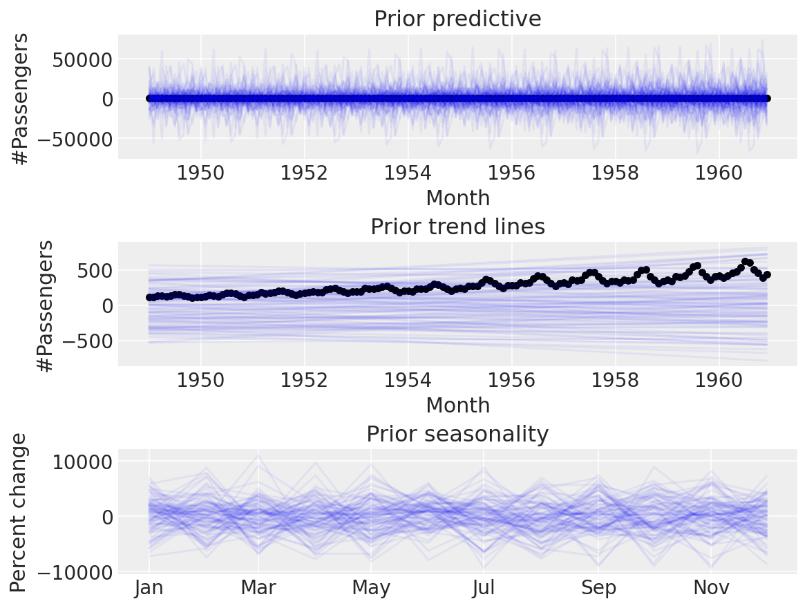
Again, this seems implausible. The default priors are too wide for our use-case, and it doesn’t make sense to use them when we can do prior predictive checks to set more sensible ones. Let’s try with some narrower ones:

coords = {"fourier_features": np.arange(2 * n_order)}
with pm.Model(check_bounds=False, coords=coords) as linear_with_seasonality:
    α = pm.Normal("α", mu=0, sigma=0.5)
    β = pm.Normal("β", mu=0, sigma=0.5)
    trend = pm.Deterministic("trend", α + β * t)

    β_fourier = pm.Normal("β_fourier", mu=0, sigma=0.1, dims="fourier_features")
    seasonality = pm.Deterministic(
        "seasonality", pm.math.dot(β_fourier, fourier_features.to_numpy().T)
    )

    μ = trend * (1 + seasonality)
    σ = pm.HalfNormal("σ", sigma=0.1)
    pm.Normal("likelihood", mu=μ, sigma=σ, observed=y)

    linear_seasonality_prior = pm.sample_prior_predictive()

fig, ax = plt.subplots(nrows=3, ncols=1, sharex=False, figsize=(8, 6))
ax[0].plot(
    df["Month"],
    az.extract_dataset(linear_seasonality_prior, group="prior_predictive", num_samples=100)[
        "likelihood"
    ]
    * y_max,
    color="blue",
    alpha=0.05,
)
df.plot.scatter(x="Month", y="#Passengers", color="k", ax=ax[0])
ax[0].set_title("Prior predictive")
ax[1].plot(
    df["Month"],
    az.extract_dataset(linear_seasonality_prior, group="prior", num_samples=100)["trend"] * y_max,
    color="blue",
    alpha=0.05,
)
df.plot.scatter(x="Month", y="#Passengers", color="k", ax=ax[1])
ax[1].set_title("Prior trend lines")
ax[2].plot(
    df["Month"].iloc[:12],
    az.extract_dataset(linear_seasonality_prior, group="prior", num_samples=100)["seasonality"][:12]
    * 100,
    color="blue",
    alpha=0.05,
)
ax[2].set_title("Prior seasonality")
ax[2].set_ylabel("Percent change")
formatter = mdates.DateFormatter("%b")
ax[2].xaxis.set_major_formatter(formatter);

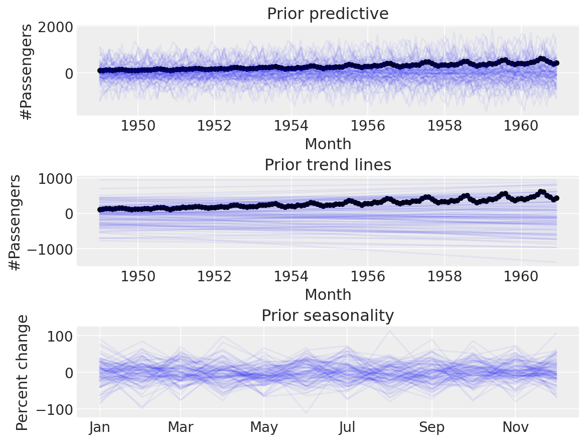
Seems a lot more believable. Time for a posterior predictive check:

with linear_with_seasonality:
    linear_seasonality_trace = pm.sample(return_inferencedata=True)
    linear_seasonality_posterior = pm.sample_posterior_predictive(trace=linear_seasonality_trace)

fig, ax = plt.subplots(nrows=3, ncols=1, sharex=False, figsize=(8, 6))
ax[0].plot(
    df["Month"],
    az.extract_dataset(linear_seasonality_posterior, group="posterior_predictive", num_samples=100)[
        "likelihood"
    ]
    * y_max,
    color="blue",
    alpha=0.05,
)
df.plot.scatter(x="Month", y="#Passengers", color="k", ax=ax[0])
ax[0].set_title("Posterior predictive")
ax[1].plot(
    df["Month"],
    az.extract_dataset(linear_trace, group="posterior", num_samples=100)["trend"] * y_max,
    color="blue",
    alpha=0.05,
)
df.plot.scatter(x="Month", y="#Passengers", color="k", ax=ax[1])
ax[1].set_title("Posterior trend lines")
ax[2].plot(
    df["Month"].iloc[:12],
    az.extract_dataset(linear_seasonality_trace, group="posterior", num_samples=100)["seasonality"][
        :12
    ]
    * 100,
    color="blue",
    alpha=0.05,
)
ax[2].set_title("Posterior seasonality")
ax[2].set_ylabel("Percent change")
formatter = mdates.DateFormatter("%b")
ax[2].xaxis.set_major_formatter(formatter);

Auto-assigning NUTS sampler...
Initializing NUTS using jitter+adapt_diag...
Multiprocess sampling (4 chains in 4 jobs)
NUTS: [α, β, β_fourier, σ]

100.00% [8000/8000 00:15<00:00 Sampling 4 chains, 0 divergences]

Sampling 4 chains for 1_000 tune and 1_000 draw iterations (4_000 + 4_000 draws total) took 16 seconds.

100.00% [4000/4000 00:00<00:00]

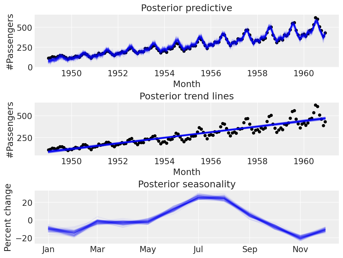
Neat!

Conclusion

We saw how we could implement a Prophet-like model ourselves and fit it to the air passengers dataset. Prophet is an awesome library and a net-positive to the community, but by implementing it ourselves, however, we can take whichever components of it we think are relevant to our problem, customise them, and carry out the Bayesian workflow [Gelman et al., 2020]). Next time you have a time series problem, I hope you will try implementing your own probabilistic model rather than using Prophet as a “black-box” whose arguments are tuneable hyperparameters.

For reference, you might also want to check out:

• TimeSeeers, a hierarchical Bayesian Time Series model based on Facebooks Prophet, written in PyMC3

• PM-Prophet, a Pymc3-based universal time series prediction and decomposition library inspired by Facebook Prophet

Authors

• Authored by Marco Gorelli in June, 2021 (pymc-examples#183)

• Updated by Danh Phan in May, 2022 (pymc-examples#320)

References

[1] (1,2)

Sean J Taylor and Benjamin Letham. Forecasting at scale. The American Statistician, 72(1):37–45, 2018. URL: https://peerj.com/preprints/3190/.

[2] (1,2)

Andrew Gelman, Aki Vehtari, Daniel Simpson, Charles C Margossian, Bob Carpenter, Yuling Yao, Lauren Kennedy, Jonah Gabry, Paul-Christian Bürkner, and Martin Modrák. Bayesian workflow. arXiv preprint arXiv:2011.01808, 2020. URL: https://arxiv.org/abs/2011.01808.

%load_ext watermark
%watermark -n -u -v -iv -w -p pytensor,aeppl,xarray

Last updated: Sun May 29 2022

Python implementation: CPython
Python version       : 3.9.12
IPython version      : 8.3.0

pytensor: 2.6.2
aeppl : 0.0.28
xarray: 2022.3.0

arviz     : 0.12.1
matplotlib: 3.5.2
pymc      : 4.0.0b6
numpy     : 1.22.4
pandas    : 1.4.2

Watermark: 2.3.0

License notice

All the notebooks in this example gallery are provided under the MIT License which allows modification, and redistribution for any use provided the copyright and license notices are preserved.

Citing PyMC examples

To cite this notebook, use the DOI provided by Zenodo for the pymc-examples repository.

Important

Many notebooks are adapted from other sources: blogs, books… In such cases you should cite the original source as well.

Also remember to cite the relevant libraries used by your code.

Here is an citation template in bibtex:

@incollection{citekey,
  author    = "<notebook authors, see above>",
  title     = "<notebook title>",
  editor    = "PyMC Team",
  booktitle = "PyMC examples",
  doi       = "10.5281/zenodo.5654871"
}

which once rendered could look like: