


Hierarchical Binomial Model: Rat Tumor Example#
import arviz as az
import matplotlib.pyplot as plt
import numpy as np
import pandas as pd
import pymc as pm
import pytensor.tensor as pt

from scipy.special import gammaln
%config InlineBackend.figure_format = 'retina'
az.style.use("arviz-variat")
This short tutorial demonstrates how to use PyMC to do inference for the rat tumour example found in chapter 5 of Bayesian Data Analysis 3rd Edition [Gelman et al., 2013]. Readers should already be familiar with the PyMC API.
Suppose we are interested in the probability that a lab rat develops endometrial stromal polyps. We have data from 71 previously performed trials and would like to use this data to perform inference.
The authors of BDA3 choose to model this problem hierarchically. Let \(y_i\) be the number of lab rats which develop endometrial stromal polyps out of a possible \(n_i\). We model the number rodents which develop endometrial stromal polyps as binomial
allowing the probability of developing an endometrial stromal polyp (i.e. \(\theta_i\)) to be drawn from some population distribution. For analytical tractability, we assume that \(\theta_i\) has Beta distribution
We are free to specify a prior distribution for \(\alpha, \beta\). We choose a weakly informative prior distribution to reflect our ignorance about the true values of \(\alpha, \beta\). The authors of BDA3 choose the joint hyperprior for \(\alpha, \beta\) to be
For more information, please see Bayesian Data Analysis 3rd Edition pg. 110.
A Directly Computed Solution#
Our joint posterior distribution is
which can be rewritten in such a way so as to obtain the marginal posterior distribution for \(\alpha\) and \(\beta\), namely
See BDA3 pg. 110 for a more information on the deriving the marginal posterior distribution. With a little determination, we can plot the marginal posterior and estimate the means of \(\alpha\) and \(\beta\) without having to resort to MCMC. We will see, however, that this requires considerable effort.
The authors of BDA3 choose to plot the surface under the parameterization \((\log(\alpha/\beta), \log(\alpha+\beta))\). We do so as well. Through the remainder of the example let \(x = \log(\alpha/\beta)\) and \(z = \log(\alpha+\beta)\).
# rat data (BDA3, p. 102)
# fmt: off
y = np.array([
    0,  0,  0,  0,  0,  0,  0,  0,  0,  0,  0,  0,  0,  0,  1,  1,  1,
    1,  1,  1,  1,  1,  2,  2,  2,  2,  2,  2,  2,  2,  2,  1,  5,  2,
    5,  3,  2,  7,  7,  3,  3,  2,  9, 10,  4,  4,  4,  4,  4,  4,  4,
    10,  4,  4,  4,  5, 11, 12,  5,  5,  6,  5,  6,  6,  6,  6, 16, 15,
    15,  9,  4
])
n = np.array([
    20, 20, 20, 20, 20, 20, 20, 19, 19, 19, 19, 18, 18, 17, 20, 20, 20,
    20, 19, 19, 18, 18, 25, 24, 23, 20, 20, 20, 20, 20, 20, 10, 49, 19,
    46, 27, 17, 49, 47, 20, 20, 13, 48, 50, 20, 20, 20, 20, 20, 20, 20,
    48, 19, 19, 19, 22, 46, 49, 20, 20, 23, 19, 22, 20, 20, 20, 52, 46,
    47, 24, 14
])
# fmt: on

N = len(n)
# Compute on log scale because products turn to sums
def log_likelihood(alpha, beta, y, n):
    LL = 0

    # Summing over data
    for Y, N in zip(y, n):
        LL += (
            gammaln(alpha + beta)
            - gammaln(alpha)
            - gammaln(beta)
            + gammaln(alpha + Y)
            + gammaln(beta + N - Y)
            - gammaln(alpha + beta + N)
        )

    return LL


def log_prior(A, B):
    return -5 / 2 * np.log(A + B)


def trans_to_beta(x, y):
    return np.exp(y) / (np.exp(x) + 1)


def trans_to_alpha(x, y):
    return np.exp(x) * trans_to_beta(x, y)


# Create space for the parameterization in which we wish to plot
X, Z = np.meshgrid(np.arange(-2.3, -1.3, 0.01), np.arange(1, 5, 0.01))
param_space = np.c_[X.ravel(), Z.ravel()]
df = pd.DataFrame(param_space, columns=["X", "Z"])

# Transform the space back to alpha beta to compute the log-posterior
df["alpha"] = trans_to_alpha(df.X, df.Z)
df["beta"] = trans_to_beta(df.X, df.Z)

df["log_posterior"] = log_prior(df.alpha, df.beta) + log_likelihood(df.alpha, df.beta, y, n)
df["log_jacobian"] = np.log(df.alpha) + np.log(df.beta)

df["transformed"] = df.log_posterior + df.log_jacobian
df["exp_trans"] = np.exp(df.transformed - df.transformed.max())

# This will ensure the density is normalized
df["normed_exp_trans"] = df.exp_trans / df.exp_trans.sum()


surface = df.set_index(["X", "Z"]).exp_trans.unstack().values.T
fig, ax = plt.subplots(figsize=(8, 8))
ax.contourf(X, Z, surface)
ax.set_xlabel(r"$\log(\alpha/\beta)$", fontsize=16)
ax.set_ylabel(r"$\log(\alpha+\beta)$", fontsize=16)

ix_z, ix_x = np.unravel_index(np.argmax(surface, axis=None), surface.shape)
ax.scatter([X[0, ix_x]], [Z[ix_z, 0]], color="red")

text = rf"$({np.round(X[0, ix_x], 2)},{np.round(Z[ix_z, 0], 2)})$"

ax.annotate(
    text,
    xy=(X[0, ix_x], Z[ix_z, 0]),
    xytext=(-1.6, 3.5),
    ha="center",
    fontsize=16,
    color="white",
    arrowprops={"facecolor": "white"},
);
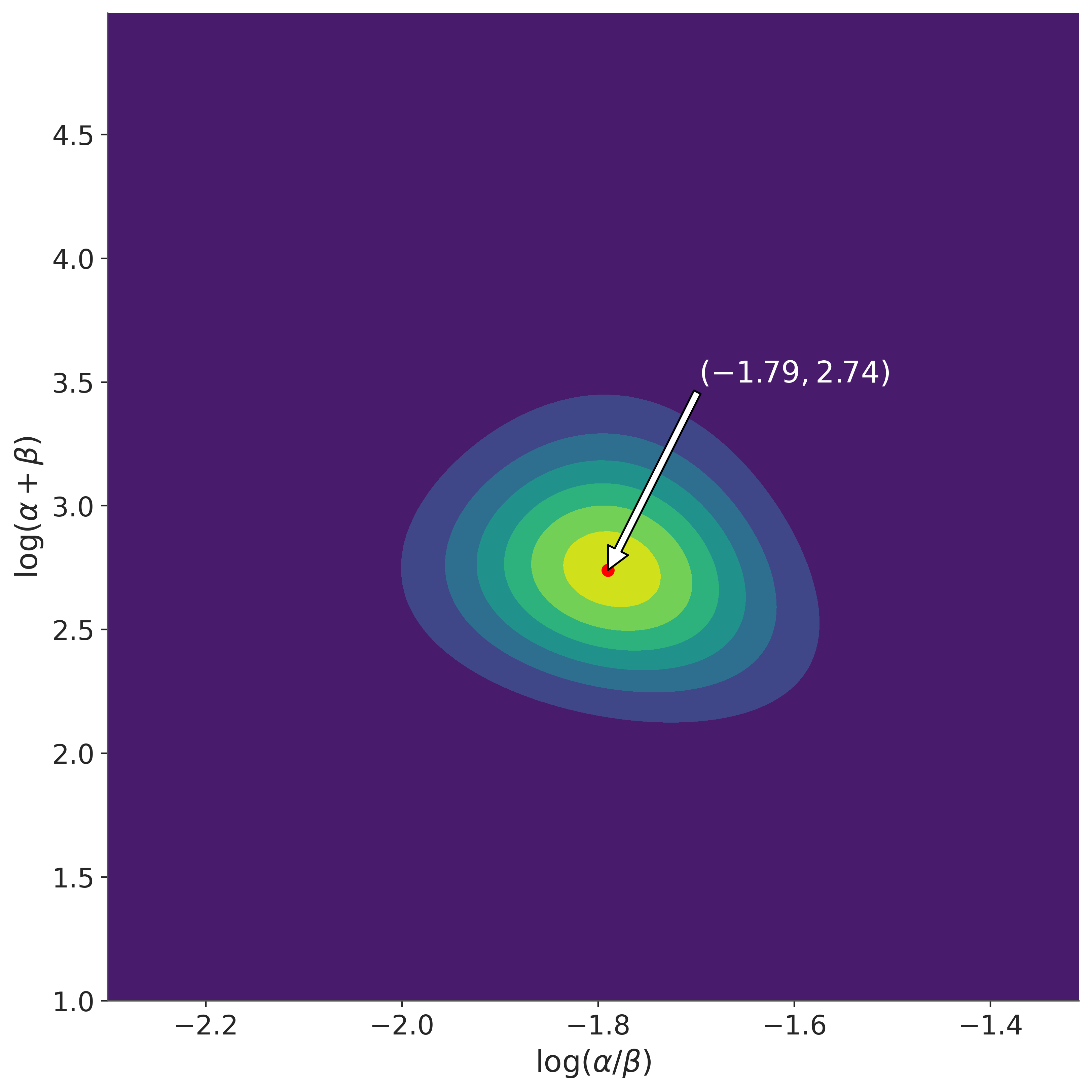
The plot shows that the posterior is roughly symmetric about the mode (-1.79, 2.74). This corresponds to \(\alpha = 2.21\) and \(\beta = 13.27\). We can compute the marginal means as the authors of BDA3 do, using
# Estimated mean of alpha
(df.alpha * df.normed_exp_trans).sum().round(3)
np.float64(2.403)
# Estimated mean of beta
(df.beta * df.normed_exp_trans).sum().round(3)
np.float64(14.319)
Computing the Posterior using PyMC#
Computing the marginal posterior directly is a lot of work, and is not always possible for sufficiently complex models.
On the other hand, creating hierarchical models in PyMC is simple. We can use the samples obtained from the posterior to estimate the means of \(\alpha\) and \(\beta\).
coords = {
    "obs_id": np.arange(N),
    "param": ["alpha", "beta"],
}
def logp_ab(value):
    """prior density"""
    return pt.log(pt.pow(pt.sum(value), -5 / 2))


with pm.Model(coords=coords) as model:
    # Uninformative prior for alpha and beta
    n_val = pm.Data("n_val", n)
    ab = pm.HalfNormal("ab", sigma=10, dims="param")
    pm.Potential("p(a, b)", logp_ab(ab))

    X = pm.Deterministic("X", pt.log(ab[0] / ab[1]))
    Z = pm.Deterministic("Z", pt.log(pt.sum(ab)))

    theta = pm.Beta("theta", alpha=ab[0], beta=ab[1], dims="obs_id")

    p = pm.Binomial("y", p=theta, observed=y, n=n_val)
    trace = pm.sample(draws=2000, tune=2000, target_accept=0.95)
Initializing NUTS using jitter+adapt_diag...
Multiprocess sampling (4 chains in 4 jobs)
NUTS: [ab, theta]
Sampling 4 chains for 2_000 tune and 2_000 draw iterations (8_000 + 8_000 draws total) took 15 seconds.
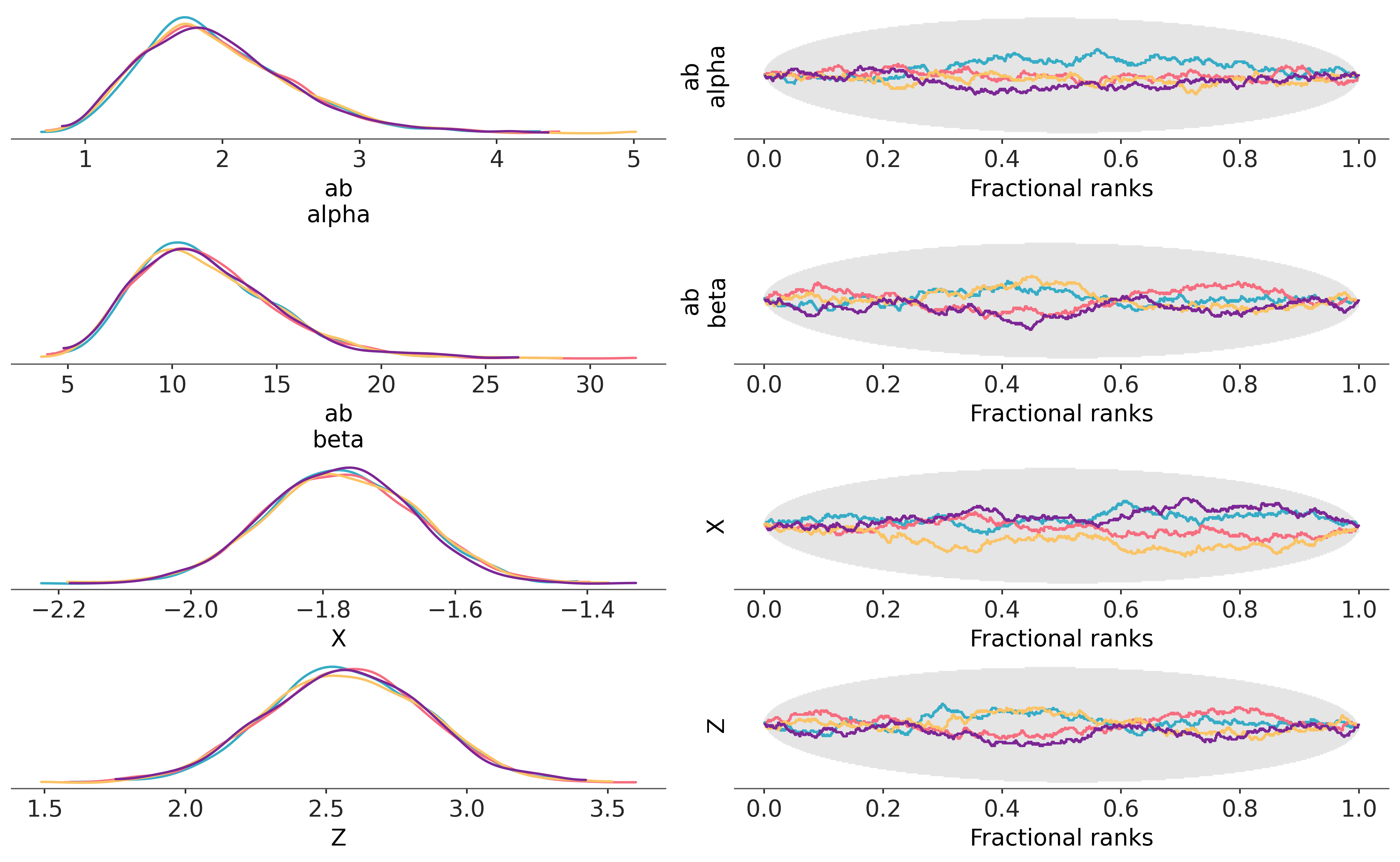
# Check the trace. Looks good!
az.plot_rank_dist(trace, var_names=["ab", "X", "Z"], compact=False);
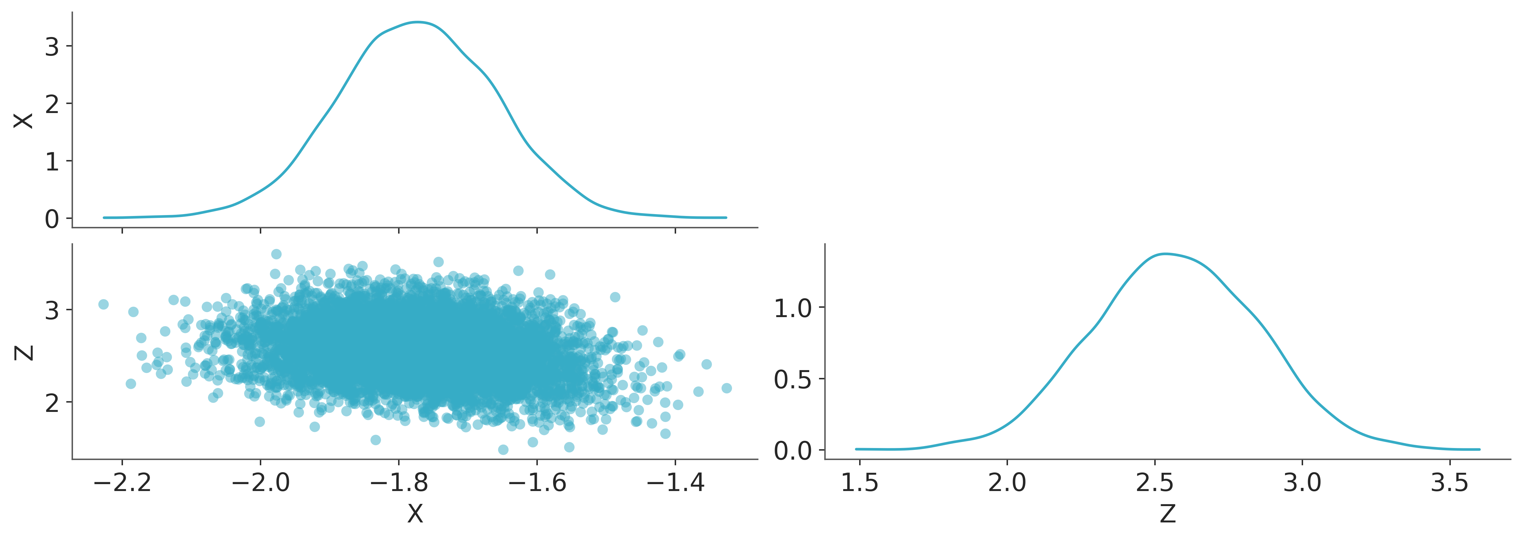
We can plot a kernel density estimate for \(x\) and \(y\). It looks rather similar to our contour plot made from the analytic marginal posterior density. That’s a good sign, and required far less effort.
az.plot_pair(trace, var_names=["X", "Z"]);
From here, we could use the trace to compute the mean of the distribution.
az.plot_dist(trace, var_names=["ab"]);
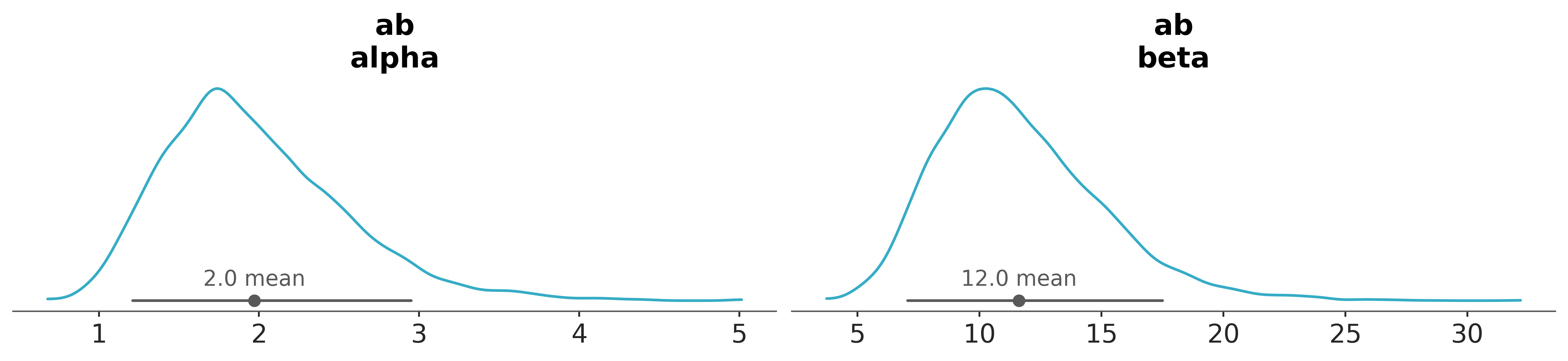
# estimate the means from the samples
trace.posterior["ab"].mean(("chain", "draw"))
<xarray.DataArray 'ab' (param: 2)> Size: 16B
array([ 1.97016693, 11.62438014])
Coordinates:
  * param    (param) <U5 40B 'alpha' 'beta'
Conclusion#
Analytically calculating statistics for posterior distributions is difficult if not impossible for some models. PyMC provides an easy way drawing samples from your model’s posterior with only a few lines of code. Here, we used PyMC to obtain estimates of the posterior mean for the rat tumor example in chapter 5 of BDA3. The estimates obtained from PyMC are encouragingly close to the estimates obtained from the analytical posterior density.
References#
Watermark#
%load_ext watermark
%watermark -n -u -v -iv -w
Last updated: Mon, 27 Apr 2026

Python implementation: CPython
Python version       : 3.14.4
IPython version      : 9.12.0

arviz     : 1.1.0
matplotlib: 3.10.8
numpy     : 2.4.4
pandas    : 3.0.2
pymc      : 5.28.0+58.gf58491a3
pytensor  : 2.38.0+133.g80cc113b5

Watermark: 2.6.0
License notice#
All the notebooks in this example gallery are provided under the MIT License which allows modification, and redistribution for any use provided the copyright and license notices are preserved.
Citing PyMC examples#
To cite this notebook, use the DOI provided by Zenodo for the pymc-examples repository.
Important
Many notebooks are adapted from other sources: blogs, books… In such cases you should cite the original source as well.
Also remember to cite the relevant libraries used by your code.
Here is an citation template in bibtex:
@incollection{citekey,
  author    = "<notebook authors, see above>",
  title     = "<notebook title>",
  editor    = "PyMC Team",
  booktitle = "PyMC examples",
  doi       = "10.5281/zenodo.5654871"
}
which once rendered could look like: