Multi-output Gaussian Processes: Coregionalization models using Hamadard product

This notebook shows how to implement the Intrinsic Coregionalization Model (ICM) and the Linear Coregionalization Model (LCM) using a Hamadard product between the Coregion kernel and input kernels. Multi-output Gaussian Process is discussed in this paper by Bonilla et al. [2007]. For further information about ICM and LCM, please check out the talk on Multi-output Gaussian Processes by Mauricio Alvarez, and his slides with more references at the last page.

The advantage of Multi-output Gaussian Processes is their capacity to simultaneously learn and infer many outputs which have the same source of uncertainty from inputs. In this example, we model the average spin rates of several pitchers in different games from a baseball dataset.

import arviz as az
import matplotlib.pyplot as plt
import numpy as np
import pandas as pd
import pymc as pm
import pytensor.tensor as pt

from pymc.gp.util import plot_gp_dist

%config InlineBackend.figure_format = 'retina'
RANDOM_SEED = 8927
rng = np.random.default_rng(RANDOM_SEED)

Preparing the data

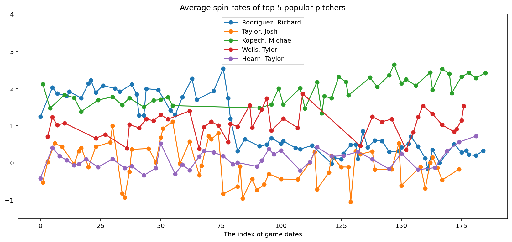
The baseball dataset contains the average spin rate of several pitchers on different game dates.

# get data
try:
    df = pd.read_csv("../data/fastball_spin_rates.csv")
except FileNotFoundError:
    df = pd.read_csv(pm.get_data("fastball_spin_rates.csv"))

print(df.shape)
df.head()

(4845, 4)

	pitcher_name	game_date	avg_spin_rate	n_pitches
0	Wainwright, Adam	2021-04-03	2127.415000	12
1	Wainwright, Adam	2021-04-08	2179.723000	11
2	Wainwright, Adam	2021-04-14	2297.968571	7
3	Wainwright, Adam	2021-04-20	2159.150000	13
4	Wainwright, Adam	2021-04-26	2314.515455	11

print(
    f"There are {df['pitcher_name'].nunique()} pitchers, in {df['game_date'].nunique()} game dates"
)

There are 262 pitchers, in 182 game dates

# Standardise average spin rate
df["avg_spin_rate"] = (df["avg_spin_rate"] - df["avg_spin_rate"].mean()) / df["avg_spin_rate"].std()
df["avg_spin_rate"].describe()

count    4.838000e+03
mean     1.821151e-16
std      1.000000e+00
min     -3.646438e+00
25%     -6.803556e-01
50%      4.736011e-03
75%      6.837128e-01
max      3.752720e+00
Name: avg_spin_rate, dtype: float64

Top N popular pitchers

# Get top N popular pitchers by who attended most games
n_outputs = 5  # Top 5 popular pitchers
top_pitchers = df.groupby("pitcher_name")["game_date"].count().nlargest(n_outputs).reset_index()
top_pitchers = top_pitchers.reset_index().rename(columns={"index": "output_idx"})
top_pitchers

	output_idx	pitcher_name	game_date
0	0	Rodriguez, Richard	64
1	1	Taylor, Josh	59
2	2	Kopech, Michael	43
3	3	Wells, Tyler	43
4	4	Hearn, Taylor	42

# Filter the data with only top N pitchers
adf = df.loc[df["pitcher_name"].isin(top_pitchers["pitcher_name"])].copy()
print(adf.shape)
adf.head()

(251, 4)

	pitcher_name	game_date	avg_spin_rate	n_pitches
1631	Rodriguez, Richard	2021-04-01	1.245044	12
1632	Rodriguez, Richard	2021-04-06	2.032285	3
1633	Rodriguez, Richard	2021-04-08	1.868068	10
1634	Rodriguez, Richard	2021-04-12	1.801864	14
1635	Rodriguez, Richard	2021-04-13	1.916592	9

adf["avg_spin_rate"].describe()

count    251.000000
mean       0.774065
std        0.867510
min       -1.050933
25%        0.102922
50%        0.559293
75%        1.517114
max        2.647740
Name: avg_spin_rate, dtype: float64

Create a game date index

# There are 142 game dates from 01 Apr 2021 to 03 Oct 2021.
adf.loc[:, "game_date"] = pd.to_datetime(adf.loc[:, "game_date"])
game_dates = adf.loc[:, "game_date"]
game_dates.min(), game_dates.max(), game_dates.nunique(), (game_dates.max() - game_dates.min())

(Timestamp('2021-04-01 00:00:00'),
 Timestamp('2021-10-03 00:00:00'),
 142,
 Timedelta('185 days 00:00:00'))

# Create a game date index
dates_idx = pd.DataFrame(
    {"game_date": pd.date_range(game_dates.min(), game_dates.max())}
).reset_index()
dates_idx = dates_idx.rename(columns={"index": "x"})
dates_idx.head()

	x	game_date
0	0	2021-04-01
1	1	2021-04-02
2	2	2021-04-03
3	3	2021-04-04
4	4	2021-04-05

Create training data

adf = adf.merge(dates_idx, how="left", on="game_date")
adf = adf.merge(top_pitchers[["pitcher_name", "output_idx"]], how="left", on="pitcher_name")
adf.head()

	pitcher_name	game_date	avg_spin_rate	n_pitches	x	output_idx
0	Rodriguez, Richard	2021-04-01	1.245044	12	0	0
1	Rodriguez, Richard	2021-04-06	2.032285	3	5	0
2	Rodriguez, Richard	2021-04-08	1.868068	10	7	0
3	Rodriguez, Richard	2021-04-12	1.801864	14	11	0
4	Rodriguez, Richard	2021-04-13	1.916592	9	12	0

adf = adf.sort_values(["output_idx", "x"])
X = adf[
    ["x", "output_idx"]
].values  # Input data includes the index of game dates, and the index of pitchers
Y = adf["avg_spin_rate"].values  # Output data includes the average spin rate of pitchers
X.shape, Y.shape

((251, 2), (251,))

Visualise training data

# Plot average spin rates of top pitchers
fig, ax = plt.subplots(1, 1, figsize=(14, 6))
legends = []
for pitcher in top_pitchers["pitcher_name"]:
    cond = adf["pitcher_name"] == pitcher
    ax.plot(adf.loc[cond, "x"], adf.loc[cond, "avg_spin_rate"], "-o")
    legends.append(pitcher)
plt.title("Average spin rates of top 5 popular pitchers")
plt.xlabel("The index of game dates")
plt.ylim([-1.5, 4.0])
plt.legend(legends, loc="upper center");

Intrinsic Coregionalization Model (ICM)

The Intrinsic Coregionalization Model (ICM) is a particular case of the Linear Coregionalization Model (LCM) with one input kernel, for example:

\[ K_{ICM} = B \otimes K_{ExpQuad} \]

Where \(B(o,o')\) is the output kernel, and \(K_{ExpQuad}(x,x')\) is an input kernel.

\[ B = WW^T + diag(kappa) \]

def get_icm(input_dim, kernel, W=None, kappa=None, B=None, active_dims=None):
    """
    This function generates an ICM kernel from an input kernel and a Coregion kernel.
    """
    coreg = pm.gp.cov.Coregion(input_dim=input_dim, W=W, kappa=kappa, B=B, active_dims=active_dims)
    icm_cov = kernel * coreg  # Use Hadamard Product for separate inputs
    return icm_cov

with pm.Model() as model:
    # Priors
    ell = pm.Gamma("ell", alpha=2, beta=0.5)
    eta = pm.Gamma("eta", alpha=3, beta=1)
    kernel = eta**2 * pm.gp.cov.ExpQuad(input_dim=2, ls=ell, active_dims=[0])
    sigma = pm.HalfNormal("sigma", sigma=3)

    # Get the ICM kernel
    W = pm.Normal("W", mu=0, sigma=3, shape=(n_outputs, 2), initval=np.random.randn(n_outputs, 2))
    kappa = pm.Gamma("kappa", alpha=1.5, beta=1, shape=n_outputs)
    B = pm.Deterministic("B", pt.dot(W, W.T) + pt.diag(kappa))
    cov_icm = get_icm(input_dim=2, kernel=kernel, B=B, active_dims=[1])

    # Define a Multi-output GP
    mogp = pm.gp.Marginal(cov_func=cov_icm)
    y_ = mogp.marginal_likelihood("f", X, Y, sigma=sigma)

pm.model_to_graphviz(model)

%%time
with model:
    gp_trace = pm.sample(2000, chains=1)

Auto-assigning NUTS sampler...
Initializing NUTS using jitter+adapt_diag...
Sequential sampling (1 chains in 1 job)
NUTS: [ell, eta, sigma, W, kappa]

100.00% [3000/3000 21:17<00:00 Sampling chain 0, 0 divergences]

Sampling 1 chain for 1_000 tune and 2_000 draw iterations (1_000 + 2_000 draws total) took 1278 seconds.

CPU times: user 46min 50s, sys: 2h 2min 57s, total: 2h 49min 47s
Wall time: 21min 25s

Prediction

# Prepare test data
M = 200  # number of data points
x_new = np.linspace(0, 200, M)[
    :, None
]  # Select 200 days (185 previous days, and add 15 days into the future).
X_new = np.vstack([x_new for idx in range(n_outputs)])
output_idx = np.vstack([np.repeat(idx, M)[:, None] for idx in range(n_outputs)])
X_new = np.hstack([X_new, output_idx])

%%time
with model:
    preds = mogp.conditional("preds", X_new)
    gp_samples = pm.sample_posterior_predictive(gp_trace, var_names=["preds"], random_seed=42)

Sampling: [preds]

100.00% [2000/2000 10:47<00:00]

CPU times: user 46min 13s, sys: 39min 48s, total: 1h 26min 2s
Wall time: 10min 50s

f_pred = gp_samples.posterior_predictive["preds"].sel(chain=0)


def plot_predictive_posteriors(f_pred, top_pitchers, M, X_new):
    fig, axes = plt.subplots(n_outputs, 1, figsize=(12, 15))

    for idx, pitcher in enumerate(top_pitchers["pitcher_name"]):
        # Prediction
        plot_gp_dist(
            axes[idx],
            f_pred[:, M * idx : M * (idx + 1)],
            X_new[M * idx : M * (idx + 1), 0],
            palette="Blues",
            fill_alpha=0.1,
            samples_alpha=0.1,
        )
        # Training data points
        cond = adf["pitcher_name"] == pitcher
        axes[idx].scatter(adf.loc[cond, "x"], adf.loc[cond, "avg_spin_rate"], color="r")
        axes[idx].set_title(pitcher)
    plt.tight_layout()


plot_predictive_posteriors(f_pred, top_pitchers, M, X_new)

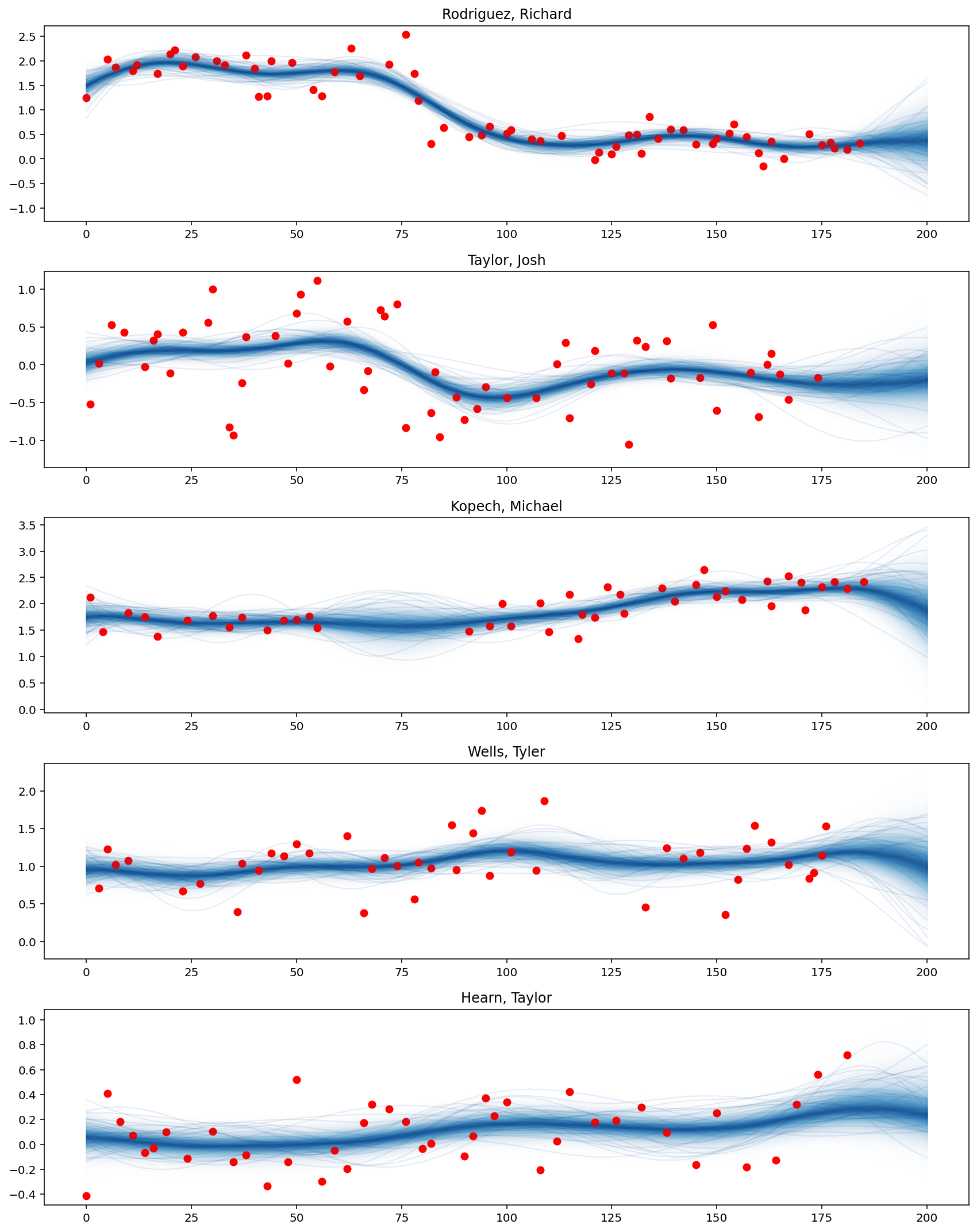
It can be seen that the average spin rate of Rodriguez Richard decreases significantly from the 75th game dates. Besides, Kopech Michael’s performance improves after a break of several weeks in the middle, while Hearn Taylor has performed better recently.

az.plot_trace(gp_trace)
plt.tight_layout()

Linear Coregionalization Model (LCM)

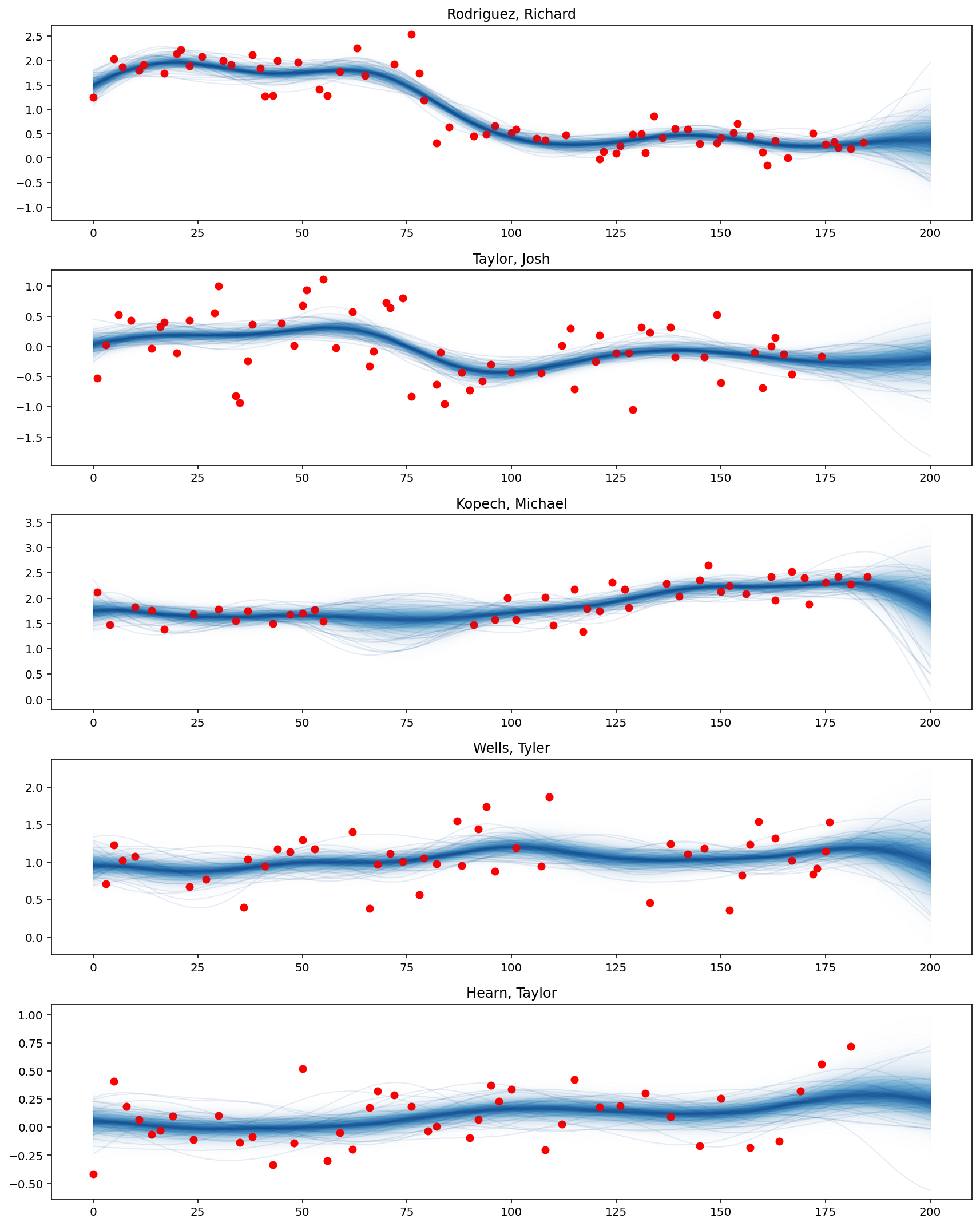
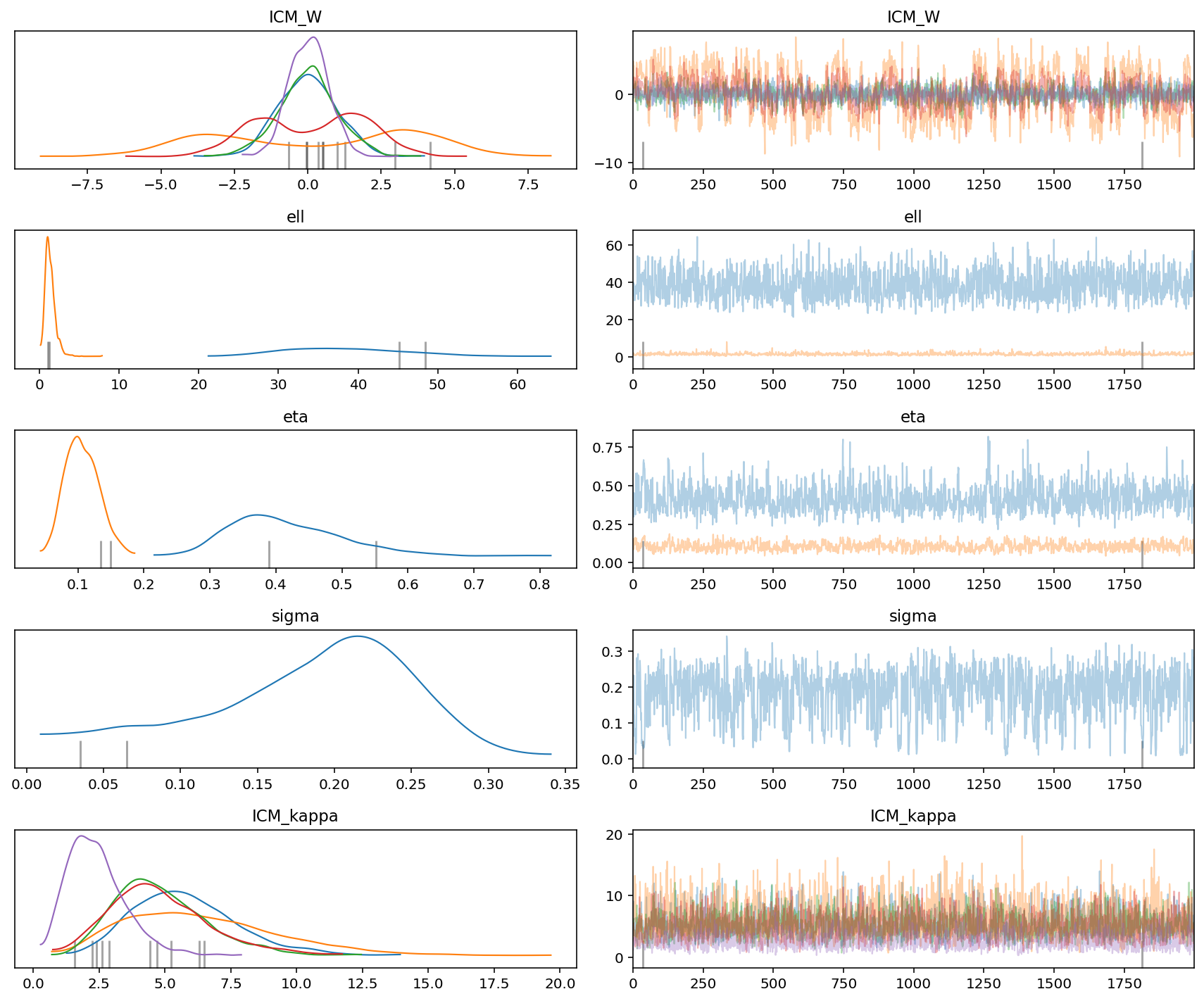
The LCM is a generalization of the ICM with two or more input kernels, so the LCM kernel is basically a sum of several ICM kernels. The LMC allows several independent samples from GPs with different covariances (kernels).

In this example, in addition to an ExpQuad kernel, we add a Matern32 kernel for input data.

\[ K_{LCM} = B \otimes K_{ExpQuad} + B \otimes K_{Matern32} \]

def get_lcm(input_dim, active_dims, num_outputs, kernels, W=None, B=None, name="ICM"):
    """
    This function generates a LCM kernel from a list of input `kernels` and a Coregion kernel.
    """
    if B is None:
        kappa = pm.Gamma(f"{name}_kappa", alpha=5, beta=1, shape=num_outputs)
        if W is None:
            W = pm.Normal(
                f"{name}_W",
                mu=0,
                sigma=5,
                shape=(num_outputs, 1),
                initval=np.random.randn(num_outputs, 1),
            )
    else:
        kappa = None

    cov_func = 0
    for idx, kernel in enumerate(kernels):
        icm = get_icm(input_dim, kernel, W, kappa, B, active_dims)
        cov_func += icm
    return cov_func

with pm.Model() as model:
    # Priors
    ell = pm.Gamma("ell", alpha=2, beta=0.5, shape=2)
    eta = pm.Gamma("eta", alpha=3, beta=1, shape=2)
    kernels = [pm.gp.cov.ExpQuad, pm.gp.cov.Matern32]
    sigma = pm.HalfNormal("sigma", sigma=3)

    # Define a list of covariance functions
    cov_list = [
        eta[idx] ** 2 * kernel(input_dim=2, ls=ell[idx], active_dims=[0])
        for idx, kernel in enumerate(kernels)
    ]

    # Get the LCM kernel
    cov_lcm = get_lcm(input_dim=2, active_dims=[1], num_outputs=n_outputs, kernels=cov_list)

    # Define a Multi-output GP
    mogp = pm.gp.Marginal(cov_func=cov_lcm)
    y_ = mogp.marginal_likelihood("f", X, Y, sigma=sigma)

pm.model_to_graphviz(model)

%%time
with model:
    gp_trace = pm.sample(2000, chains=1)

Auto-assigning NUTS sampler...
Initializing NUTS using jitter+adapt_diag...
Sequential sampling (1 chains in 1 job)
NUTS: [ell, eta, sigma, ICM_kappa, ICM_W]

100.00% [3000/3000 18:28<00:00 Sampling chain 0, 2 divergences]

Sampling 1 chain for 1_000 tune and 2_000 draw iterations (1_000 + 2_000 draws total) took 1109 seconds.
There were 2 divergences after tuning. Increase `target_accept` or reparameterize.

CPU times: user 40min 37s, sys: 1h 47min 9s, total: 2h 27min 46s
Wall time: 18min 39s

Prediction

%%time
with model:
    preds = mogp.conditional("preds", X_new)
    gp_samples = pm.sample_posterior_predictive(gp_trace, var_names=["preds"], random_seed=42)

Sampling: [preds]

100.00% [2000/2000 12:50<00:00]

CPU times: user 51min 44s, sys: 50min 14s, total: 1h 41min 59s
Wall time: 12min 53s

plot_predictive_posteriors(f_pred, top_pitchers, M, X_new)

az.plot_trace(gp_trace)
plt.tight_layout()

Acknowledgement

This work is supported by 2022 Google Summer of Codes and NUMFOCUS.

Authors

• Authored by Danh Phan, Bill Engels, Chris Fonnesbeck in November, 2022 (pymc-examples#454)

References

[1]

Edwin V Bonilla, Kian Chai, and Christopher Williams. Multi-task gaussian process prediction. Advances in neural information processing systems, 2007. URL: https://papers.nips.cc/paper/2007/hash/66368270ffd51418ec58bd793f2d9b1b-Abstract.html.

Watermark

%load_ext watermark
%watermark -n -u -v -iv -w -p pytensor,aeppl,xarray

The watermark extension is already loaded. To reload it, use:
  %reload_ext watermark
Last updated: Sat Nov 12 2022

Python implementation: CPython
Python version       : 3.9.12
IPython version      : 8.3.0

pytensor: 2.8.6
aeppl : 0.0.36
xarray: 2022.3.0

pymc      : 4.2.1
arviz     : 0.13.0
pandas    : 1.4.2
pytensor    : 2.8.6
numpy     : 1.22.4
matplotlib: 3.5.2

Watermark: 2.3.0

License notice

All the notebooks in this example gallery are provided under the MIT License which allows modification, and redistribution for any use provided the copyright and license notices are preserved.

Citing PyMC examples

To cite this notebook, use the DOI provided by Zenodo for the pymc-examples repository.

Important

Many notebooks are adapted from other sources: blogs, books… In such cases you should cite the original source as well.

Also remember to cite the relevant libraries used by your code.

Here is an citation template in bibtex:

@incollection{citekey,
  author    = "<notebook authors, see above>",
  title     = "<notebook title>",
  editor    = "PyMC Team",
  booktitle = "PyMC examples",
  doi       = "10.5281/zenodo.5654871"
}

which once rendered could look like: