Assurance Planning via Simulation

The experimentation lifecycle as a Bosch triptych. Left, Bayesian Assurance (this notebook): before any data arrive, the planner reads possible effects from the prior and asks what the experiment will likely conclude. Centre, Sensitivity Analysis: a single experiment is wracked by the biases it cannot rule out, and the model is contorted to see which commitments its conclusion can survive. Right, Meta-Analysis: many experiments are pooled through a hierarchy of levels into a synthesis that becomes the next plan’s prior. Three panels, one posterior machinery.

Experimental questions are seeded in the science that preceded them. Answers are stress-tested and refined. New experiments spawn further questions again. This is the cycle.

The question planners are actually asking

When we experiment, we encode questions. Implicitly we assume an answer will be useful. Our hypotheses are “operationalised” as power heuristics: given an effect size, what is the probability we cross a fixed threshold? This is an indirect and contorted gauge of efficacy. Instead of asking whether the treatment is effective, we often ask whether the results are surprising assuming a degree of effectiveness. The slippage between these two questions has produced a generation of experimental plans calibrated to invented effect sizes rather than to the beliefs the planners actually hold.

An alternative is Bayesian Assurance. The construction is mechanical: draw from the priors, generate a dataset, fit the treatment model, apply the decision rule, repeat. The result is a single number: the probability the experiment will conclude what its stakeholders need. The process is the same whether the response is continuous (like revenue per visitor) or binary (like conversion); we develop it on the Gaussian case first and confirm the process is invariant to the response scale. This notebook is the first of three on the lifecycle of a Bayesian experiment; see Sensitivity Analysis for Unmeasured Confounding for the interpretation counterpart and Multiple Experiments and Bayesian Meta-analysis for the synthesis counterpart. The same inferential machinery serves all three panels of the triptych, but what changes is the problem put to it.

Where this lands in regulatory practice

We are going to apply Bayesian assurance to a question in product-analytics but the technique has a wider application. The FDA’s 2026 draft guidance on Bayesian methodology in clinical trials defines Bayesian power as the probability of meeting the success criterion averaged over a prior distribution [U.S. Food and Drug Administration, 2026], which is assurance under another name. The FDA guidance formalises the success rule as \(\Pr(\text{effect} > a) > c\) (the rule used below, with \(a = 0\) and \(c = 0.95\)). The same guidance separates the design prior that generates the synthetic trials from the analysis prior used in inference. The generative and inference models below are distinct objects for this reason. Below we’ll runs the assurance loop with the two priors deliberately mismatched. The clinical trial setting in the FDA report differs from product experimentation; the machinery is identical.

import warnings

from dataclasses import dataclass

import arviz as az
import matplotlib.pyplot as plt
import matplotlib.ticker as mticker
import numpy as np
import pandas as pd
import pymc as pm

from scipy import stats

warnings.filterwarnings("ignore", category=RuntimeWarning)
warnings.filterwarnings("ignore", category=UserWarning)

%config InlineBackend.figure_format = 'retina'
az.style.use("arviz-variat")
rng = np.random.default_rng(42)
RANDOM_SEED = 42

The scenario

An e-commerce team is evaluating a redesigned checkout flow. We cover two outcomes: the continuous outcome is revenue per visitor, the binary outcome is conversion. We will not commit to a particular vertical or product; the structure is generic to any A/B test with one of these outcome types. What matters is that the same prior beliefs and the same decision rule will be asked of two different likelihoods. The Gaussian case will carry the argument; the Bernoulli case will confirm it travels.

@dataclass
class EffectPrior:
    """Prior beliefs about a treatment effect, on the scale of the outcome."""

    mu: float
    sigma: float

    def sample(self, rng, size=1):
        return rng.normal(self.mu, self.sigma, size=size)

Power and assurance: two questions, different focus

Power and assurance share an interface and answer different questions. Power conditions on a specific effect size \(\theta_0\) that the planner has been pressed into naming, and computes the probability of rejecting the null at that value:

\[ \text{Power}(N) = P\!\left(\text{reject } H_0 \mid \theta = \theta_0,\; N\right). \]

The conditioning bar is the load-bearing part. The planner who has confidently named \(\theta_0\) has implicitly used up the uncertainty that motivated the experiment in the first place. Assurance refuses the substitution. Instead it integrates over the planner’s prior beliefs about the effect. The decision rule is whether the posterior probability of a positive effect clears a threshold \(c\):

\[\begin{split} \text{Assurance}(N) = \mathbb{E}_{\substack{\theta \,\sim\, \pi(\theta) \\ \hat{d} \,\sim\, p(\hat{d} \mid \theta,\, N)}}\!\left[\mathbb{1}\!\bigl(P(\theta > 0 \mid \hat{d},\, N) > c\bigr)\right]. \end{split}\]

The outer expectation averages over effect sizes drawn from the prior; the inner averages over data generated under each effect ([O'Hagan et al., 2005], [Spiegelhalter et al., 2004]). The integration is the entire move. Where power asks the planner to invent a world, assurance asks them to describe the one they already believe they are in. With that description in place, we can quantify how likely the result is when conditioned on the prior distribution.

The simulation engine

Assurance is an expectation over the prior predictive distribution: the joint distribution of effect and data that the model generates before any real data arrive. As a Monte Carlo estimator the integral becomes a procedure in three steps, repeated for each candidate sample size:

1. Sample the prior predictive of an unconditioned generative model. Each draw is a complete synthetic experiment: an effect drawn from the prior, and a dataset of size \(N\) generated under it.

2. Fit the analysis model to each synthetic dataset and apply the decision rule.

3. Record the fraction of synthetic experiments in which the decision succeeded.

Drawing a truth and generating data under it is exactly what pm.sample_prior_predictive does on a model with no observed data, so we let PyMC’s generative machinery produce the synthetic experiments rather than hand-rolling the sampling with numpy. The generative model that produces the data and the inference model that analyses it are separate objects, and keeping them separate is the point: the generative model encodes the worlds we are planning for, the inference model encodes how we will reason once real data arrive. This workflow is defined as a function and passed through a sample size grid to determine how many N is required to achieve surety in the finding.

def assurance_curve(assurance_fn, N_grid, n_sims, rng, **kwargs):
    """Estimate the assurance curve by evaluating assurance at each sample size."""
    records = []
    for N in N_grid:
        a = assurance_fn(N=int(N), n_sims=n_sims, rng=rng, **kwargs)
        records.append({"N": int(N), "assurance": a})
    return pd.DataFrame(records)

Gaussian outcome: revenue per visitor

The Gaussian case is the cleanest place to make the mechanics explicit. Each arm produces a revenue-per-visitor outcome with known noise scale \(\sigma_{\text{obs}}\) (we treat this as known here; in practice it is estimated from a pilot or historical data). The team is interested in the treatment effect \(\delta = \mu_B - \mu_A\), and holds a prior over \(\delta\) informed by past experiments in similar product surfaces. That prior is not conjured from nothing: Multiple Experiments and Bayesian Meta-analysis shows how a meta-analysis of past experiments produces exactly this kind of prior, so the synthesis at the end of one experiment’s lifecycle is the planning input at the start of the next. Concretely, the meta-analytic predictive there closes on \(\mathcal{N}(0.4, 0.5)\), which is exactly the EFFECT_PRIOR defined below: the number that ends that notebook opens this one.

Two models do the work. The generative model is unconditioned: it places the planning prior on \(\delta\) and generates synthetic datasets, and it is the object we hand to pm.sample_prior_predictive. The inference model conditions on a dataset and returns the posterior on \(\delta\); the decision rule asks whether the posterior probability of a positive effect exceeds a threshold (0.95 below). For the assurance loop the conjugate Normal–Normal posterior on \(\delta\) admits a closed form, which lets us evaluate the decision on each synthetic experiment without running MCMC every time.

We will verify that closed form against the inference model’s MCMC posterior at a single sample size before relying on it. This also underwrites the idea that we can use MCMC for this procedure even with more complex models.

SIGMA_OBS = 4.0
DECISION_THRESHOLD = 0.95
BASELINE_REVENUE = 10.0
# Not free-floating: this is the meta-analytic predictive for a new market from
# the synthesis notebook (meta_analysis_experiments), which closes on N(0.4, 0.5).
EFFECT_PRIOR = EffectPrior(mu=0.4, sigma=0.5)


def gaussian_generative_model(N, prior):
    """Unconditioned model: planning prior on the effect plus the data-generating likelihood."""
    with pm.Model() as model:
        delta = pm.Normal("delta", mu=prior.mu, sigma=prior.sigma)
        pm.Normal("y_A", mu=BASELINE_REVENUE, sigma=SIGMA_OBS, shape=N)
        pm.Normal("y_B", mu=BASELINE_REVENUE + delta, sigma=SIGMA_OBS, shape=N)
    return model


def gaussian_two_arm_model(y_A, y_B, prior):
    """Inference model: conditions on an observed dataset and returns the posterior on the effect."""
    with pm.Model() as model:
        mu_A = pm.Normal("mu_A", mu=BASELINE_REVENUE, sigma=5.0)
        delta = pm.Normal("delta", mu=prior.mu, sigma=prior.sigma)
        mu_B = pm.Deterministic("mu_B", mu_A + delta)
        pm.Normal("obs_A", mu=mu_A, sigma=SIGMA_OBS, observed=y_A)
        pm.Normal("obs_B", mu=mu_B, sigma=SIGMA_OBS, observed=y_B)
    return model

A single synthetic experiment makes the inference model concrete. We use the do-operator to fix the generative effect at a chosen value, draw one dataset from the prior predictive, and condition the inference model on it.

demo_true_delta = 0.6
demo_model = pm.do(gaussian_generative_model(N=200, prior=EFFECT_PRIOR), {"delta": demo_true_delta})
demo_draw = pm.sample_prior_predictive(1, model=demo_model, random_seed=RANDOM_SEED)
y_A_demo = demo_draw.prior["y_A"].values.reshape(-1)
y_B_demo = demo_draw.prior["y_B"].values.reshape(-1)

with gaussian_two_arm_model(y_A_demo, y_B_demo, EFFECT_PRIOR):
    idata_gauss_demo = pm.sample(
        draws=1000,
        tune=1000,
        chains=2,
        target_accept=0.95,
        random_seed=RANDOM_SEED,
        progressbar=False,
    )

Sampling: [y_A, y_B]
NUTS[nutpie]: [mu_A, delta]

pc = az.plot_dist(
    idata_gauss_demo,
    var_names=["delta"],
    visuals={"title": {"text": r"Posterior on $\delta$ at $N=200$ (one simulated dataset)"}},
)
az.add_lines(
    pc,
    values=0.0,
    visuals={"ref_line": {"color": "C1", "label": "ref = 0.0"}},
)
pc.get_viz("plot").legend();

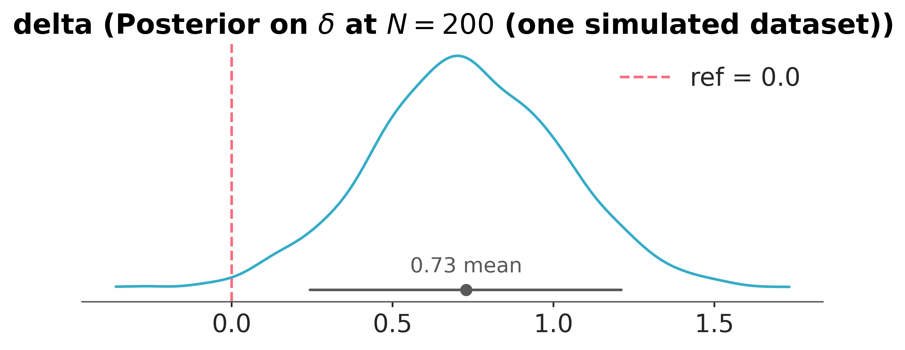
The posterior concentrates above zero; under the decision rule the team would conclude the new flow lifts revenue. That is a single draw of the experiment. Assurance asks how often this conclusion would arrive if we re-ran the experiment many times under our actual prior.

The conjugate posterior on \(\delta\) given \(\hat d = \bar y_B - \bar y_A\) has mean and variance:

\[ \sigma_d^2 = \frac{2\sigma_{\text{obs}}^2}{N}, \quad \tau^2_{\text{post}} = \left(\frac{1}{\tau_0^2} + \frac{1}{\sigma_d^2}\right)^{-1}, \quad \mu_{\text{post}} = \tau^2_{\text{post}}\left(\frac{\mu_0}{\tau_0^2} + \frac{\hat d}{\sigma_d^2}\right), \]

where \((\mu_0, \tau_0)\) is the prior on \(\delta\). We check this matches the PyMC posterior before relying on it.

def gaussian_posterior_delta(d_hat, N, sigma_obs, prior):
    sigma_d_sq = 2 * sigma_obs**2 / N
    post_var = 1.0 / (1.0 / prior.sigma**2 + 1.0 / sigma_d_sq)
    post_mean = post_var * (prior.mu / prior.sigma**2 + d_hat / sigma_d_sq)
    return post_mean, np.sqrt(post_var)


d_hat_demo = y_B_demo.mean() - y_A_demo.mean()
analytical_mu, analytical_sd = gaussian_posterior_delta(
    d_hat_demo, N=200, sigma_obs=SIGMA_OBS, prior=EFFECT_PRIOR
)
mcmc_mu = idata_gauss_demo.posterior["delta"].mean().item()
mcmc_sd = idata_gauss_demo.posterior["delta"].std().item()

pd.DataFrame(
    {"analytical": [analytical_mu, analytical_sd], "MCMC": [mcmc_mu, mcmc_sd]},
    index=["posterior mean of delta", "posterior sd of delta"],
).round(3)

	analytical	MCMC
posterior mean of delta	0.745	0.728
posterior sd of delta	0.312	0.303

The two posteriors agree to within MCMC noise. Now we get to the heart of the technique and push our procedure through different sample values of N.

def gaussian_assurance_at_N(N, n_sims, prior, sigma_obs, threshold, rng, analysis_prior=None):
    # `prior` is the design prior: it generates the synthetic worlds. `analysis_prior`
    # is used to form the posterior; it defaults to the design prior so a single
    # argument reproduces the matched-prior case.
    analysis_prior = prior if analysis_prior is None else analysis_prior
    seed = int(rng.integers(2**31 - 1))
    pp = pm.sample_prior_predictive(
        n_sims, model=gaussian_generative_model(N, prior), random_seed=seed
    )
    y_A = pp.prior["y_A"].values.reshape(n_sims, N)
    y_B = pp.prior["y_B"].values.reshape(n_sims, N)
    d_hat = y_B.mean(axis=1) - y_A.mean(axis=1)
    post_mu, post_sd = gaussian_posterior_delta(d_hat, N, sigma_obs, analysis_prior)
    prob_positive = 1.0 - stats.norm.cdf(0.0, loc=post_mu, scale=post_sd)
    return float((prob_positive > threshold).mean())


N_GRID = np.array([100, 200, 400, 800, 1600, 3200, 6400])
N_SIMS = 1000

assurance_df = assurance_curve(
    gaussian_assurance_at_N,
    N_grid=N_GRID,
    n_sims=N_SIMS,
    rng=np.random.default_rng(RANDOM_SEED),
    prior=EFFECT_PRIOR,
    sigma_obs=SIGMA_OBS,
    threshold=DECISION_THRESHOLD,
)
assurance_df

Sampling: [delta, y_A, y_B]
Sampling: [delta, y_A, y_B]
Sampling: [delta, y_A, y_B]
Sampling: [delta, y_A, y_B]
Sampling: [delta, y_A, y_B]
Sampling: [delta, y_A, y_B]
Sampling: [delta, y_A, y_B]

	N	assurance
0	100	0.267
1	200	0.398
2	400	0.501
3	800	0.603
4	1600	0.640
5	3200	0.681
6	6400	0.717

For each simulated future dataset, we compute the posterior distribution of the treatment effect and evaluate the posterior probability that the effect is positive, prob_positive. A trial is considered decisive if prob_positive exceeds the pre-specified DECISION_THRESHOLD. The Bayesian assurance is the proportion of simulated trials that satisfy this decision criterion. As the planned sample size increases, posterior uncertainty decreases, leading to a larger proportion of decisive trials and therefore higher assurance.

For comparison we compute frequentist power at a single fixed effect size. The convention is to set the effect to the prior mean, which is itself an arbitrary choice, and a revealing one.

def gaussian_power(N, delta_alt, sigma_obs, alpha=0.05):
    sigma_d = np.sqrt(2 * sigma_obs**2 / N)
    z_crit = stats.norm.ppf(1 - alpha)
    return 1.0 - stats.norm.cdf(z_crit - delta_alt / sigma_d)


power_at_prior_mean = np.array([gaussian_power(N, EFFECT_PRIOR.mu, SIGMA_OBS) for N in N_GRID])
power_at_optimistic = np.array(
    [gaussian_power(N, EFFECT_PRIOR.mu + EFFECT_PRIOR.sigma, SIGMA_OBS) for N in N_GRID]
)
power_at_pessimistic = np.array(
    [gaussian_power(N, max(EFFECT_PRIOR.mu - EFFECT_PRIOR.sigma, 0.01), SIGMA_OBS) for N in N_GRID]
)

prior_prob_positive = 1.0 - stats.norm.cdf(0.0, EFFECT_PRIOR.mu, EFFECT_PRIOR.sigma)

fig, ax = plt.subplots(figsize=(15, 5.5))
ax.plot(N_GRID, assurance_df["assurance"], marker="o", linewidth=2, label="Assurance (Bayesian)")
ax.plot(
    N_GRID,
    power_at_prior_mean,
    marker="s",
    linestyle="--",
    label=r"Power at $\theta_0 = \mu_{\text{prior}}$",
)
ax.plot(
    N_GRID,
    power_at_optimistic,
    marker="^",
    linestyle=":",
    alpha=0.7,
    label=r"Power at $\mu + \sigma$",
)
ax.plot(
    N_GRID,
    power_at_pessimistic,
    marker="v",
    linestyle=":",
    alpha=0.7,
    label=r"Power at $\mu - \sigma$",
)
ax.axhline(
    prior_prob_positive,
    color="C0",
    linestyle="-.",
    alpha=0.6,
    label=rf"Assurance ceiling $P(\delta>0)$ = {prior_prob_positive:.2f}",
)
ax.set_xscale("log")
ax.xaxis.set_major_formatter(mticker.FuncFormatter(lambda x, _: f"{int(x):,}"))
ax.set_xlabel("Sample size per arm")
ax.set_ylabel("Probability of declaring uplift")
ax.set_title("Assurance vs frequentist power, Gaussian outcome")
ax.legend(loc="lower right", fontsize=9);

The three power curves fan out because each conditions on a single assumed world. Power at \(\mu + \sigma\) assumes an effect of \(0.9\) and saturates almost immediately; power at \(\mu - \sigma\) is pinned near the test’s five-percent floor, because \(\mu - \sigma\) lands at essentially zero effect, where even large samples gain almost no detection. Power at the prior mean is the curve a frequentist planner would actually quote. The assurance curve is the prior-weighted integral across the entire fan, and it tells a different story than any single power calculation.

The story is in the crossing. Between \(N=400\) and \(N=800\) the assurance curve drops below power-at-the-mean, having sat above it at smaller samples. At small samples assurance is buoyed by the optimistic tail of the prior: it counts the plausible draws above \(0.4\), effects of \(0.8\) or \(1.0\) that even a hundred observations have a real chance of detecting, which the single-point power calculation never sees. Quoting power at the mean understates what small experiments can do, because it ignores the optimistic tail of the prior that assurance counts.

At large samples the relationship inverts, and the reason is the ceiling drawn above. Power at a fixed positive effect climbs to one: with enough data an effect of \(0.4\) is certain to be detected. Assurance cannot reach one: the prior assigns positive probability to a zero or negative effect. Its asymptote is exactly the prior probability that the effect is beneficial, \(P(\delta > 0) \approx 0.79\). No sample size buys more assurance than \(P(\delta > 0)\). A planner should know that ceiling before committing to more data, and no point on a power curve reveals it.

The minimum detectable effect leads a double life

Power is usually quoted at a “minimum detectable effect” (MDE), and that single number carries more weight than it appears to. Read one way, the MDE is a utility threshold: an effect smaller than this is not worth shipping, so failing to detect it does not matter, and powering at the MDE is a coherent design target. Read another way, it is a forecast: a quiet assumption that the true effect is about this large and positive, sometimes reverse-engineered from the sample size a team can already afford. The frequentist machinery itself is innocent here, because the false-positive rate \(\alpha\) already governs the null case; it is the floor that the \(\mu - \sigma\) curve traces. What conditions the null away is the reported summary, “\(X\%\) power to detect the MDE”, which is computed entirely inside the world where the effect is real and exactly the MDE. Assurance does not abolish this assumption. It relocates it from an implicit point to an explicit prior, where the probability that the effect is null or harmful becomes visible and open to argument.

The same machinery on a binary outcome

The generative model fixes the baseline conversion rate, places the planning prior on the lift, and emits binomial counts per arm. The inference step places Beta priors on the per-arm rates and reads off the posterior probability that the lift is positive ([Stucchio, 2015], [Kruschke, 2014]).

BASELINE_RATE = 0.10
RATE_LIFT_PRIOR = EffectPrior(mu=0.005, sigma=0.012)
BETA_PRIOR_KAPPA = 200  # prior concentration, in units of pseudo-observations
prior_prob_lift_positive = 1.0 - stats.norm.cdf(0.0, RATE_LIFT_PRIOR.mu, RATE_LIFT_PRIOR.sigma)


def beta_prior_params(p_mean, kappa):
    return kappa * p_mean, kappa * (1 - p_mean)


def bernoulli_generative_model(N, rate_prior, baseline_rate):
    """Unconditioned model: fixed baseline rate, planning prior on the lift, binomial counts per arm."""
    with pm.Model() as model:
        lift = pm.Normal("lift", mu=rate_prior.mu, sigma=rate_prior.sigma)
        p_B = pm.Deterministic("p_B", pm.math.clip(baseline_rate + lift, 1e-4, 1 - 1e-4))
        pm.Binomial("n_A", n=N, p=baseline_rate)
        pm.Binomial("n_B", n=N, p=p_B)
    return model


def bernoulli_assurance_at_N(
    N, n_sims, rate_prior, baseline_rate, kappa, threshold, rng, n_post=2000
):
    seed = int(rng.integers(2**31 - 1))
    pp = pm.sample_prior_predictive(
        n_sims,
        model=bernoulli_generative_model(N, rate_prior, baseline_rate),
        random_seed=seed,
    )
    n_A = pp.prior["n_A"].values.reshape(-1).astype(int)
    n_B = pp.prior["n_B"].values.reshape(-1).astype(int)
    actual_sims = len(n_A)  # PyMC v6 may return fewer draws than requested
    alpha0, beta0 = beta_prior_params(baseline_rate, kappa)
    p_A_post = rng.beta(alpha0 + n_A[:, None], beta0 + N - n_A[:, None], size=(actual_sims, n_post))
    p_B_post = rng.beta(alpha0 + n_B[:, None], beta0 + N - n_B[:, None], size=(actual_sims, n_post))
    prob_positive = (p_B_post > p_A_post).mean(axis=1)
    return float((prob_positive > threshold).mean())

N_GRID_BERN = np.array([500, 1000, 2000, 4000, 8000, 16000, 32000])

assurance_bern_df = assurance_curve(
    bernoulli_assurance_at_N,
    N_grid=N_GRID_BERN,
    n_sims=N_SIMS,
    rng=np.random.default_rng(RANDOM_SEED),
    rate_prior=RATE_LIFT_PRIOR,
    baseline_rate=BASELINE_RATE,
    kappa=BETA_PRIOR_KAPPA,
    threshold=DECISION_THRESHOLD,
)


def bernoulli_power(N, p_A, lift_alt, alpha=0.05):
    p_B = p_A + lift_alt
    p_bar = 0.5 * (p_A + p_B)
    se_null = np.sqrt(2 * p_bar * (1 - p_bar) / N)
    se_alt = np.sqrt(p_A * (1 - p_A) / N + p_B * (1 - p_B) / N)
    z_crit = stats.norm.ppf(1 - alpha)
    return 1.0 - stats.norm.cdf((z_crit * se_null - lift_alt) / se_alt)


power_bern_at_prior_mean = np.array(
    [bernoulli_power(N, BASELINE_RATE, RATE_LIFT_PRIOR.mu) for N in N_GRID_BERN]
)
power_bern_at_optimistic = np.array(
    [
        bernoulli_power(N, BASELINE_RATE, RATE_LIFT_PRIOR.mu + RATE_LIFT_PRIOR.sigma)
        for N in N_GRID_BERN
    ]
)
power_bern_at_pessimistic = np.array(
    [
        bernoulli_power(N, BASELINE_RATE, max(RATE_LIFT_PRIOR.mu - RATE_LIFT_PRIOR.sigma, 1e-4))
        for N in N_GRID_BERN
    ]
)

fig, ax = plt.subplots(figsize=(15, 4.5))
ax.plot(
    N_GRID_BERN,
    assurance_bern_df["assurance"],
    marker="o",
    linewidth=2,
    label="Assurance (Bayesian)",
)
ax.plot(
    N_GRID_BERN,
    power_bern_at_prior_mean,
    marker="s",
    linestyle="--",
    label=r"Power at lift $=\mu_{\text{prior}}$",
)
ax.plot(
    N_GRID_BERN,
    power_bern_at_optimistic,
    marker="^",
    linestyle=":",
    alpha=0.7,
    label=r"Power at $\mu + \sigma$",
)
ax.plot(
    N_GRID_BERN,
    power_bern_at_pessimistic,
    marker="v",
    linestyle=":",
    alpha=0.7,
    label=r"Power at $\mu - \sigma$",
)
ax.axhline(
    prior_prob_lift_positive,
    color="C0",
    linestyle="-.",
    alpha=0.6,
    label=rf"Assurance ceiling $P(\text{{lift}}>0)$ = {prior_prob_lift_positive:.2f}",
)

ax.set_xscale("log")
ax.xaxis.set_major_formatter(mticker.FuncFormatter(lambda x, _: f"{int(x):,}"))
ax.set_xlabel("Sample size per arm")
ax.set_ylabel("Probability of declaring uplift")
ax.set_title("Assurance vs frequentist power, Bernoulli outcome")
ax.legend(loc="lower right");

Sampling: [lift, n_A, n_B]
Sampling: [lift, n_A, n_B]
Sampling: [lift, n_A, n_B]
Sampling: [lift, n_A, n_B]
Sampling: [lift, n_A, n_B]
Sampling: [lift, n_A, n_B]
Sampling: [lift, n_A, n_B]

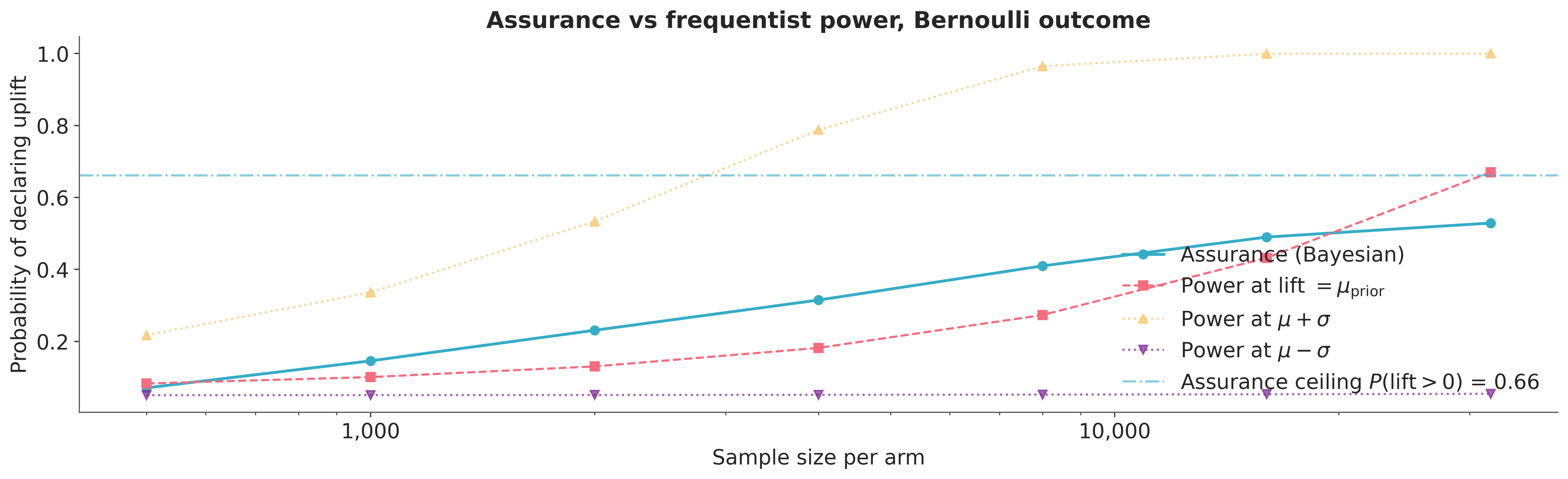
The conversion-rate version runs the same loop, and the loop discloses something the Gaussian case conceals. The lift is bounded above: how large a positive effect can even be depends on how much room sits above the baseline conversion rate, a constraint the Normal likelihood never faces. The Beta prior on the per-arm rates is parameterised here by a concentration \(\kappa\), the number of pseudo-observations at the baseline rate that the prior is equivalent to. Setting \(\kappa = 200\) is saying: I am as confident about the baseline as if I had watched 200 trials at that rate. This is a different handle on prior calibration than the Normal’s mean and standard deviation pair, and it makes the ceiling claim more precise: the assurance curve asymptotes toward the prior probability that the lift is positive, and what that probability is depends not only on the prior’s location and scale but on the scale on which the lift is defined. At a 10% baseline with a planning prior mean of 0.5%, the prior splits its mass roughly two to one in favour of a positive lift, and the assurance curve asymptotes there, near 0.66. The same machinery produces a lower ceiling than the Gaussian case because the planning prior commits to a more cautious belief about how large a conversion lift can plausibly be. The generative model produced the synthetic experiments; the conjugate Beta posterior supplied the decision, with no MCMC in the loop. We confirm below that this matches a full PyMC fit on a single dataset, so nothing in the assurance machinery depends on the closed form being available; it depends only on a posterior we can compute reliably.

def bernoulli_two_arm_model(n_A, n_B, N, baseline_rate, kappa):
    alpha0, beta0 = beta_prior_params(baseline_rate, kappa)
    with pm.Model() as model:
        p_A = pm.Beta("p_A", alpha=alpha0, beta=beta0)
        p_B = pm.Beta("p_B", alpha=alpha0, beta=beta0)
        pm.Deterministic("lift", p_B - p_A)
        pm.Binomial("obs_A", n=N, p=p_A, observed=n_A)
        pm.Binomial("obs_B", n=N, p=p_B, observed=n_B)
    return model


demo_model_bern = pm.do(
    bernoulli_generative_model(N=4000, rate_prior=RATE_LIFT_PRIOR, baseline_rate=BASELINE_RATE),
    {"lift": 0.015},
)
demo_draw_bern = pm.sample_prior_predictive(1, model=demo_model_bern, random_seed=RANDOM_SEED)
n_A_demo = int(demo_draw_bern.prior["n_A"].values.reshape(-1)[0])
n_B_demo = int(demo_draw_bern.prior["n_B"].values.reshape(-1)[0])

with bernoulli_two_arm_model(
    n_A_demo, n_B_demo, N=4000, baseline_rate=BASELINE_RATE, kappa=BETA_PRIOR_KAPPA
):
    idata_bern_demo = pm.sample(
        draws=1000,
        tune=1000,
        target_accept=0.95,
        random_seed=RANDOM_SEED,
        progressbar=False,
    )

pc = az.plot_dist(
    idata_bern_demo,
    var_names=["lift"],
    visuals={"title": {"text": r"Posterior on conversion lift at $N=4000$"}},
)
az.add_lines(
    pc,
    values=0.0,
    visuals={"ref_line": {"color": "C1", "label": "ref = 0.0"}},
)
pc.get_viz("plot").legend()

Sampling: [n_A, n_B]
NUTS[nutpie]: [p_A, p_B]

<matplotlib.legend.Legend at 0x35447ae90>

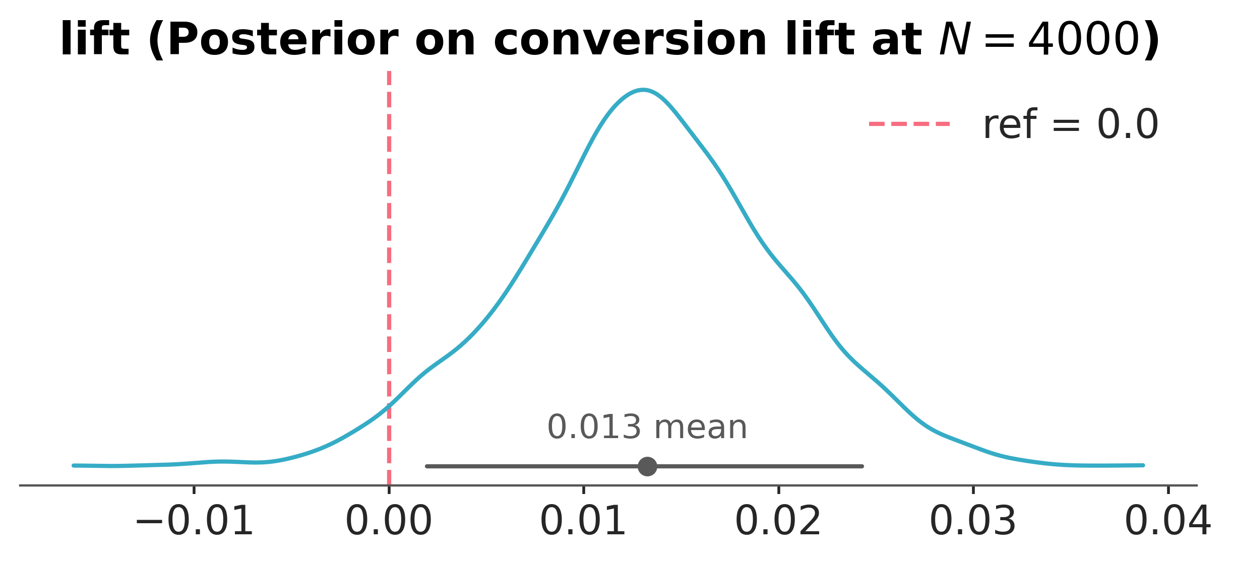
The PyMC posterior on lift agrees with the conjugate Beta posterior, as it must under this setup. The decision rule is the same, and the ceiling is lower because the planning prior carries a smaller probability that the lift is positive. That prior probability sets the asymptote that no sample size can exceed.

The cost of an under-informed prior

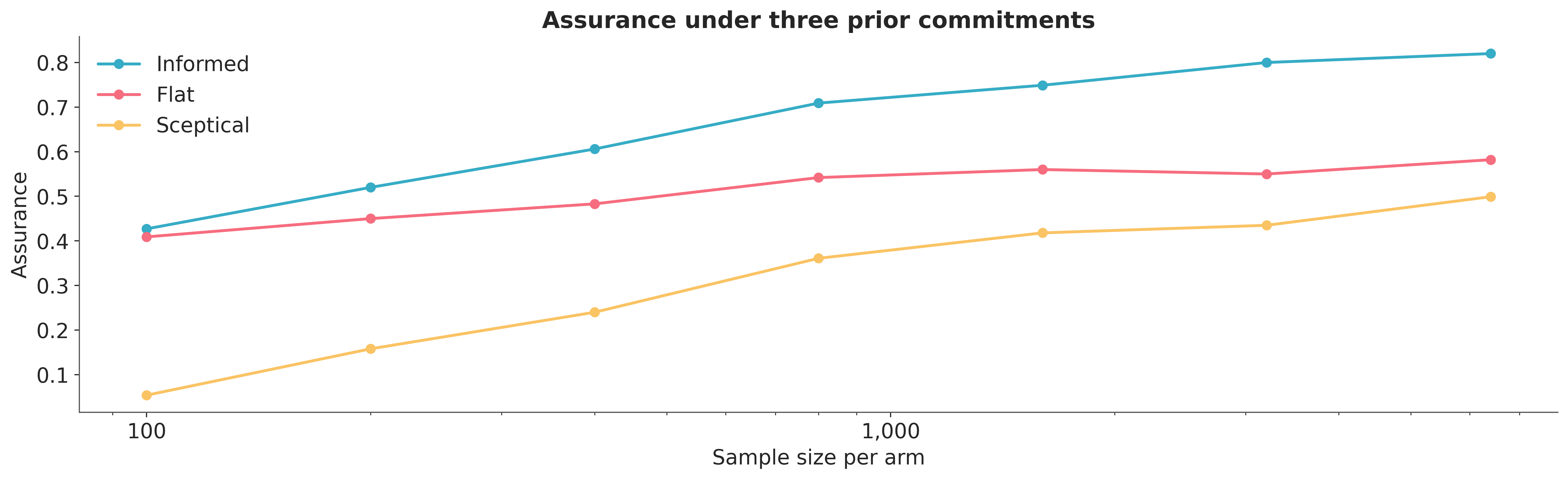
The assurance curve is conditional on the prior. A tightly informative prior centred near the truth produces an optimistic-looking curve; a flat prior produces a curve that requires substantially more data to reach the same assurance. Neither is wrong. They report what each prior commitment buys the planner.

INFORMED_PRIOR = EffectPrior(mu=0.4, sigma=0.3)
FLAT_PRIOR = EffectPrior(mu=0.4, sigma=1.5)
SCEPTICAL_PRIOR = EffectPrior(mu=0.1, sigma=0.5)

prior_comparison = {}
for name, prior in [
    ("Informed", INFORMED_PRIOR),
    ("Flat", FLAT_PRIOR),
    ("Sceptical", SCEPTICAL_PRIOR),
]:
    df = assurance_curve(
        gaussian_assurance_at_N,
        N_grid=N_GRID,
        n_sims=N_SIMS,
        rng=np.random.default_rng(RANDOM_SEED),
        prior=prior,
        sigma_obs=SIGMA_OBS,
        threshold=DECISION_THRESHOLD,
    )
    prior_comparison[name] = df

fig, ax = plt.subplots(figsize=(15, 4.5))
for name, df in prior_comparison.items():
    ax.plot(df["N"], df["assurance"], marker="o", linewidth=2, label=name)
ax.set_xscale("log")
ax.xaxis.set_major_formatter(mticker.FuncFormatter(lambda x, _: f"{int(x):,}"))
ax.set_xlabel("Sample size per arm")
ax.set_ylabel("Assurance")
ax.set_title("Assurance under three prior commitments")
ax.legend();

Sampling: [delta, y_A, y_B]
Sampling: [delta, y_A, y_B]
Sampling: [delta, y_A, y_B]
Sampling: [delta, y_A, y_B]
Sampling: [delta, y_A, y_B]
Sampling: [delta, y_A, y_B]
Sampling: [delta, y_A, y_B]
Sampling: [delta, y_A, y_B]
Sampling: [delta, y_A, y_B]
Sampling: [delta, y_A, y_B]
Sampling: [delta, y_A, y_B]
Sampling: [delta, y_A, y_B]
Sampling: [delta, y_A, y_B]
Sampling: [delta, y_A, y_B]
Sampling: [delta, y_A, y_B]
Sampling: [delta, y_A, y_B]
Sampling: [delta, y_A, y_B]
Sampling: [delta, y_A, y_B]
Sampling: [delta, y_A, y_B]
Sampling: [delta, y_A, y_B]
Sampling: [delta, y_A, y_B]

Design prior and analysis prior

The assurance loop carries two priors with distinct jobs. The design prior generates the synthetic worlds the experiment will face. The analysis prior reads each dataset and forms the posterior the decision rule consults. Every curve so far set the two equal. Separating them measures a sensitivity the FDA guidance asks for directly: how the operating characteristics respond when the inference commitment disagrees with the planning belief [U.S. Food and Drug Administration, 2026]. The generative model already carries the design prior and the inference model the analysis prior, so the loop runs the mismatch with one extra argument.

OPTIMISTIC_DESIGN = EffectPrior(mu=0.6, sigma=0.4)
SCEPTICAL_ANALYSIS = EffectPrior(mu=0.0, sigma=0.3)

design_analysis_cases = {
    "Matched (design = analysis)": (OPTIMISTIC_DESIGN, OPTIMISTIC_DESIGN),
    "Optimistic design, sceptical analysis": (OPTIMISTIC_DESIGN, SCEPTICAL_ANALYSIS),
    "Sceptical design, optimistic analysis": (SCEPTICAL_ANALYSIS, OPTIMISTIC_DESIGN),
}

design_analysis_curves = {}
for name, (design_prior, analysis_prior) in design_analysis_cases.items():
    design_analysis_curves[name] = assurance_curve(
        gaussian_assurance_at_N,
        N_grid=N_GRID,
        n_sims=N_SIMS,
        rng=np.random.default_rng(RANDOM_SEED),
        prior=design_prior,
        analysis_prior=analysis_prior,
        sigma_obs=SIGMA_OBS,
        threshold=DECISION_THRESHOLD,
    )

fig, ax = plt.subplots(figsize=(15, 4.5))
for name, df in design_analysis_curves.items():
    ax.plot(df["N"], df["assurance"], marker="o", linewidth=2, label=name)
ax.set_xscale("log")
ax.xaxis.set_major_formatter(mticker.FuncFormatter(lambda x, _: f"{int(x):,}"))
ax.set_xlabel("Sample size per arm")
ax.set_ylabel("Assurance")
ax.set_title("Assurance when the design and analysis priors agree or disagree")
ax.legend();

Sampling: [delta, y_A, y_B]
Sampling: [delta, y_A, y_B]
Sampling: [delta, y_A, y_B]
Sampling: [delta, y_A, y_B]
Sampling: [delta, y_A, y_B]
Sampling: [delta, y_A, y_B]
Sampling: [delta, y_A, y_B]
Sampling: [delta, y_A, y_B]
Sampling: [delta, y_A, y_B]
Sampling: [delta, y_A, y_B]
Sampling: [delta, y_A, y_B]
Sampling: [delta, y_A, y_B]
Sampling: [delta, y_A, y_B]
Sampling: [delta, y_A, y_B]
Sampling: [delta, y_A, y_B]
Sampling: [delta, y_A, y_B]
Sampling: [delta, y_A, y_B]
Sampling: [delta, y_A, y_B]
Sampling: [delta, y_A, y_B]
Sampling: [delta, y_A, y_B]
Sampling: [delta, y_A, y_B]

A sceptical analysis prior lowers assurance at every sample size, because it discounts the same evidence the optimistic design prior expects to see. The reverse pairing recovers most of the matched curve once the data accumulate, since an optimistic analysis prior and a growing dataset agree. The gap between the curves is the price of a mismatch, and it narrows as \(N\) grows. Small experiments pay the most for an analysis prior that disagrees with the design belief, which matches the guidance observation that trial characteristics are most sensitive to the analysis prior when the sample size is small [U.S. Food and Drug Administration, 2026].

The information content of a prior: effective sample size

The three curves above differ because the three priors carry different amounts of information. The prior effective sample size (ESS) makes this precise: it is the number of actual experimental observations the prior is equivalent to in terms of information content. A prior with ESS of 128 is, before the first participant is enrolled, already as informative as 128 observed subjects per arm.

For the two-arm Gaussian trial the ESS follows from equating information in the prior with information from \(n\) observations. The prior \(\mathcal{N}(\mu_0, \sigma_0^2)\) carries information \(1/\sigma_0^2\); the effect estimate from \(n\) observations carries \(n / 2\sigma_{\text{obs}}^2\). Setting them equal:

\[n_{\text{ESS}} = \frac{2\sigma_{\text{obs}}^2}{\sigma_0^2}\]

The simulation-based approach recovers the same number without the closed form. For each \(N\) in a grid, draw synthetic datasets from the prior predictive and compute the posterior variance under a flat reference prior; the \(N^*\) where the average posterior variance crosses the prior variance is the ESS. The machinery is the same prior-predictive loop already running in the assurance calculation; only the inner step changes. In the conjugate case the analytical posterior fills that step. In non-conjugate models such as hierarchical likelihoods or logistic regression, the same loop runs with MCMC posteriors and the ESS estimate generalises without modification. Verifying that analytical and simulation estimates agree for the Gaussian case validates the approach for those more complex settings.

def analytical_ess(prior, sigma_obs):
    """Prior ESS for a two-arm Gaussian trial: 2σ²_obs / σ²_prior."""
    return 2 * sigma_obs**2 / prior.sigma**2


pd.DataFrame(
    {
        "prior_mu": [p.mu for p in [INFORMED_PRIOR, EFFECT_PRIOR, FLAT_PRIOR, SCEPTICAL_PRIOR]],
        "prior_sigma": [
            p.sigma for p in [INFORMED_PRIOR, EFFECT_PRIOR, FLAT_PRIOR, SCEPTICAL_PRIOR]
        ],
        "analytical_ESS": [
            analytical_ess(p, SIGMA_OBS)
            for p in [INFORMED_PRIOR, EFFECT_PRIOR, FLAT_PRIOR, SCEPTICAL_PRIOR]
        ],
    },
    index=["Informed", "Default", "Flat", "Sceptical"],
).round(1)

	prior_mu	prior_sigma	analytical_ESS
Informed	0.4	0.3	355.6
Default	0.4	0.5	128.0
Flat	0.4	1.5	14.2
Sceptical	0.1	0.5	128.0

def simulation_based_ess(prior, sigma_obs, N_grid, n_sims, rng):
    """
    Estimate prior ESS via simulation: find N* where the mean posterior variance
    under a flat reference prior crosses the prior variance.

    Uses the same prior-predictive sampling as the assurance loop. Replace
    gaussian_posterior_delta with an MCMC posterior to extend to non-conjugate models.
    """
    flat_ref = EffectPrior(mu=0.0, sigma=10 * sigma_obs)
    target_var = prior.sigma**2
    records = []
    for N in N_grid:
        N = int(N)
        seed = int(rng.integers(2**31 - 1))
        pp = pm.sample_prior_predictive(
            n_sims, model=gaussian_generative_model(N, prior), random_seed=seed
        )
        y_A = pp.prior["y_A"].values.reshape(n_sims, N)
        y_B = pp.prior["y_B"].values.reshape(n_sims, N)
        d_hat = y_B.mean(axis=1) - y_A.mean(axis=1)
        _, post_sd = gaussian_posterior_delta(d_hat, N, sigma_obs, flat_ref)
        records.append({"N": N, "mean_post_var": float(np.mean(post_sd**2))})
    df = pd.DataFrame(records)
    post_vars = df["mean_post_var"].values
    N_vals = df["N"].values.astype(float)
    # post_var decreases with N; interpolate to find where it crosses the prior variance
    ess_sim = float(np.interp(target_var, post_vars[::-1], N_vals[::-1]))
    return ess_sim, df


N_ESS_GRID = np.unique(np.round(np.geomspace(10, 600, 30)).astype(int))
N_ESS_SIMS = 200
ess_rng = np.random.default_rng(RANDOM_SEED + 99)

ess_results = {}
for name, prior in [
    ("Informed", INFORMED_PRIOR),
    ("Default", EFFECT_PRIOR),
    ("Flat", FLAT_PRIOR),
    ("Sceptical", SCEPTICAL_PRIOR),
]:
    ess_a = analytical_ess(prior, SIGMA_OBS)
    ess_s, df_curve = simulation_based_ess(prior, SIGMA_OBS, N_ESS_GRID, N_ESS_SIMS, ess_rng)
    ess_results[name] = {
        "prior": prior,
        "ess_analytical": ess_a,
        "ess_sim": ess_s,
        "curve": df_curve,
    }

pd.DataFrame(
    {
        "prior_sigma": {n: v["prior"].sigma for n, v in ess_results.items()},
        "analytical_ESS": {n: round(v["ess_analytical"], 1) for n, v in ess_results.items()},
        "simulation_ESS": {n: round(v["ess_sim"], 1) for n, v in ess_results.items()},
    }
)

Sampling: [delta, y_A, y_B]
Sampling: [delta, y_A, y_B]
Sampling: [delta, y_A, y_B]
Sampling: [delta, y_A, y_B]
Sampling: [delta, y_A, y_B]
Sampling: [delta, y_A, y_B]
Sampling: [delta, y_A, y_B]
Sampling: [delta, y_A, y_B]
Sampling: [delta, y_A, y_B]
Sampling: [delta, y_A, y_B]
Sampling: [delta, y_A, y_B]
Sampling: [delta, y_A, y_B]
Sampling: [delta, y_A, y_B]
Sampling: [delta, y_A, y_B]
Sampling: [delta, y_A, y_B]
Sampling: [delta, y_A, y_B]
Sampling: [delta, y_A, y_B]
Sampling: [delta, y_A, y_B]
Sampling: [delta, y_A, y_B]
Sampling: [delta, y_A, y_B]
Sampling: [delta, y_A, y_B]
Sampling: [delta, y_A, y_B]
Sampling: [delta, y_A, y_B]
Sampling: [delta, y_A, y_B]
Sampling: [delta, y_A, y_B]
Sampling: [delta, y_A, y_B]
Sampling: [delta, y_A, y_B]
Sampling: [delta, y_A, y_B]
Sampling: [delta, y_A, y_B]
Sampling: [delta, y_A, y_B]
Sampling: [delta, y_A, y_B]
Sampling: [delta, y_A, y_B]
Sampling: [delta, y_A, y_B]
Sampling: [delta, y_A, y_B]
Sampling: [delta, y_A, y_B]
Sampling: [delta, y_A, y_B]
Sampling: [delta, y_A, y_B]
Sampling: [delta, y_A, y_B]
Sampling: [delta, y_A, y_B]
Sampling: [delta, y_A, y_B]
Sampling: [delta, y_A, y_B]
Sampling: [delta, y_A, y_B]
Sampling: [delta, y_A, y_B]
Sampling: [delta, y_A, y_B]
Sampling: [delta, y_A, y_B]
Sampling: [delta, y_A, y_B]
Sampling: [delta, y_A, y_B]
Sampling: [delta, y_A, y_B]
Sampling: [delta, y_A, y_B]
Sampling: [delta, y_A, y_B]
Sampling: [delta, y_A, y_B]
Sampling: [delta, y_A, y_B]
Sampling: [delta, y_A, y_B]
Sampling: [delta, y_A, y_B]
Sampling: [delta, y_A, y_B]
Sampling: [delta, y_A, y_B]
Sampling: [delta, y_A, y_B]
Sampling: [delta, y_A, y_B]
Sampling: [delta, y_A, y_B]
Sampling: [delta, y_A, y_B]
Sampling: [delta, y_A, y_B]
Sampling: [delta, y_A, y_B]
Sampling: [delta, y_A, y_B]
Sampling: [delta, y_A, y_B]
Sampling: [delta, y_A, y_B]
Sampling: [delta, y_A, y_B]
Sampling: [delta, y_A, y_B]
Sampling: [delta, y_A, y_B]
Sampling: [delta, y_A, y_B]
Sampling: [delta, y_A, y_B]
Sampling: [delta, y_A, y_B]
Sampling: [delta, y_A, y_B]
Sampling: [delta, y_A, y_B]
Sampling: [delta, y_A, y_B]
Sampling: [delta, y_A, y_B]
Sampling: [delta, y_A, y_B]
Sampling: [delta, y_A, y_B]
Sampling: [delta, y_A, y_B]
Sampling: [delta, y_A, y_B]
Sampling: [delta, y_A, y_B]
Sampling: [delta, y_A, y_B]
Sampling: [delta, y_A, y_B]
Sampling: [delta, y_A, y_B]
Sampling: [delta, y_A, y_B]
Sampling: [delta, y_A, y_B]
Sampling: [delta, y_A, y_B]
Sampling: [delta, y_A, y_B]
Sampling: [delta, y_A, y_B]
Sampling: [delta, y_A, y_B]
Sampling: [delta, y_A, y_B]
Sampling: [delta, y_A, y_B]
Sampling: [delta, y_A, y_B]
Sampling: [delta, y_A, y_B]
Sampling: [delta, y_A, y_B]
Sampling: [delta, y_A, y_B]
Sampling: [delta, y_A, y_B]
Sampling: [delta, y_A, y_B]
Sampling: [delta, y_A, y_B]
Sampling: [delta, y_A, y_B]
Sampling: [delta, y_A, y_B]
Sampling: [delta, y_A, y_B]
Sampling: [delta, y_A, y_B]
Sampling: [delta, y_A, y_B]
Sampling: [delta, y_A, y_B]
Sampling: [delta, y_A, y_B]
Sampling: [delta, y_A, y_B]
Sampling: [delta, y_A, y_B]
Sampling: [delta, y_A, y_B]
Sampling: [delta, y_A, y_B]
Sampling: [delta, y_A, y_B]
Sampling: [delta, y_A, y_B]
Sampling: [delta, y_A, y_B]
Sampling: [delta, y_A, y_B]
Sampling: [delta, y_A, y_B]
Sampling: [delta, y_A, y_B]
Sampling: [delta, y_A, y_B]
Sampling: [delta, y_A, y_B]
Sampling: [delta, y_A, y_B]
Sampling: [delta, y_A, y_B]
Sampling: [delta, y_A, y_B]

	prior_sigma	analytical_ESS	simulation_ESS
Informed	0.3	355.6	357.1
Default	0.5	128.0	128.1
Flat	1.5	14.2	14.3
Sceptical	0.5	128.0	128.1

fig, axes = plt.subplots(1, 2, figsize=(20, 5))

# Left: ESS crossing picture for the default prior
res = ess_results["Default"]
curve = res["curve"]
prior_d = res["prior"]
ess_a_d = res["ess_analytical"]
ess_s_d = res["ess_sim"]

axes[0].plot(
    curve["N"],
    curve["mean_post_var"],
    marker="o",
    color="C0",
    markersize=4,
    label="Mean posterior variance (flat prior)",
)
axes[0].axhline(
    prior_d.sigma**2,
    color="C3",
    linestyle="--",
    label=rf"Prior variance $\sigma_0^2$ = {prior_d.sigma**2:.2f}",
)
axes[0].axvline(
    ess_a_d,
    color="C2",
    linestyle=":",
    linewidth=2,
    label=f"Analytical ESS = {ess_a_d:.0f}",
)
axes[0].axvline(
    ess_s_d,
    color="C3",
    linestyle=":",
    linewidth=2,
    alpha=0.7,
    label=f"Simulation ESS ≈ {ess_s_d:.0f}",
)
axes[0].set_xlabel("N per arm")
axes[0].set_ylabel("Mean posterior variance under flat prior")
axes[0].set_title(r"ESS crossing: default prior ($\sigma_0 = 0.5$)")
axes[0].legend()

# Right: assurance curves with ESS positions annotated
for name in ["Informed", "Flat", "Sceptical"]:
    res = ess_results[name]
    df = prior_comparison[name]
    ess_a = res["ess_analytical"]
    axes[1].plot(
        df["N"],
        df["assurance"],
        marker="o",
        linewidth=2,
        label=f"{name} (ESS ≈ {ess_a:.0f})",
    )
    axes[1].axvline(ess_a, linestyle=":", alpha=0.35)

axes[1].set_xscale("log")
axes[1].xaxis.set_major_formatter(mticker.FuncFormatter(lambda x, _: f"{int(x):,}"))
axes[1].set_xlabel("Sample size per arm")
axes[1].set_ylabel("Assurance")
axes[1].set_title("Assurance curves with ESS marked")
axes[1].legend();

The left panel is a calibration check. The simulation curve, posterior variance under a flat prior as a function of N, crosses the prior variance at the point the analytical formula predicts. The two estimates agree to within interpolation noise. For non-conjugate models where no closed form for the posterior variance exists, the same loop with MCMC posteriors in place of gaussian_posterior_delta gives the correct ESS. The conjugate case validates the simulation approach before the closed form disappears.

The right panel reads the ESS against the assurance curves. The dotted vertical lines mark each prior’s ESS on the sample-size axis. An ESS of 356 (Informed) means the prior carries more information than 350 subjects per arm before the first participant is enrolled; the curve climbs steeply early because the prior is already doing most of the work. An ESS of 14 (Flat) means the prior contributes almost nothing, and every observation earns its full weight. The ESS converts the abstract question “how informative is this prior?” into a number on the same axis as the assurance curve: experiments whose planned N falls well below the ESS are prior-dominated; those well above it are data-dominated.

This is the quantitative form of the trade-off the sensitivity analysis in Sensitivity Analysis for Unmeasured Confounding interrogates from the other side. There, the question is what happens when that committed information meets an identification gap, and the tipping point at which the conclusion turns measures how much that committed ESS has put at risk.

The three curves disagree most where they should: at small sample sizes where the data has not yet overwhelmed the prior. The informed prior reaches high assurance fastest because it is willing to commit to a narrow effect range; the sceptical prior assumes a smaller effect and so needs more data to detect it; the flat prior carries enough probability mass over zero that even moderate datasets do not push the posterior reliably above the decision threshold. The point is to make the dependence of the assurance number on the prior commitment visible, so the prior becomes a subject of negotiation rather than a hidden choice.

Planning as a posterior over future posteriors

The experiment we have not yet run is a posterior we have not yet computed. What we have is a prior, a model, and the patience to ask what the experiment will likely say.

Statistical power questions answers a conditional: given a specific effect, what probability of detection? Bayesian assurance answers a marginal question: given everything currently believed, what probability that the inference about to be drawn will be useful? The operation that produces assurance is the same one that will produce the posterior at the end of the experiment - only the data are still hypothetical. Assurance makes explicit the assumption power leaves buried, a believed distribution of effects, and derives from that assumption a posterior to evaluate.

The Gaussian case and the Bernoulli case ran the same inference machinery. What changed was the likelihood, and with it the ceiling its geometry sets on how much assurance any sample size can buy. The next notebook, Sensitivity Analysis for Unmeasured Confounding, keeps the machinery and changes the question: not what an experiment will probably say, but what it did say once clean identification is itself in doubt.

Authors

• Authored by Nathaniel Forde in May 2026.

References

[1] (1,2,3)

U.S. Food and Drug Administration. Use of bayesian methodology in clinical trials of drug and biological products: guidance for industry (draft guidance). Draft Guidance, Center for Drug Evaluation and Research (CDER) and Center for Biologics Evaluation and Research (CBER), January 2026. Distributed for comment purposes only.

[2]

Anthony O'Hagan, John W. Stevens, and Michael J. Campbell. Assurance in clinical trial design. Pharmaceutical Statistics, 4(3):187–201, 2005. doi:10.1002/pst.175.

[3]

David J. Spiegelhalter, Keith R. Abrams, and Jonathan P. Myles. Bayesian Approaches to Clinical Trials and Health-Care Evaluation. John Wiley & Sons, 2004.

[4]

Chris Stucchio. Bayesian a/b testing at vwo. 2015. URL: https://vwo.com/downloads/VWO_SmartStats_technical_whitepaper.pdf.

[5]

John Kruschke. Doing Bayesian data analysis: A tutorial with R, JAGS, and Stan. Academic Press, 2014.

Watermark

%load_ext watermark
%watermark -n -u -v -iv -w -p pytensor,xarray

Last updated: Mon, 29 Jun 2026

Python implementation: CPython
Python version       : 3.13.13
IPython version      : 9.14.0

pytensor: 3.0.3
xarray  : 2026.4.0

arviz     : 1.1.0
matplotlib: 3.10.9
numpy     : 2.3.5
pandas    : 2.3.3
pymc      : 6.0.1
scipy     : 1.17.1

Watermark: 2.6.0

License notice

All the notebooks in this example gallery are provided under the MIT License which allows modification, and redistribution for any use provided the copyright and license notices are preserved.

Citing PyMC examples

To cite this notebook, use the DOI provided by Zenodo for the pymc-examples repository.

Important

Many notebooks are adapted from other sources: blogs, books… In such cases you should cite the original source as well.

Also remember to cite the relevant libraries used by your code.

Here is an citation template in bibtex:

@incollection{citekey,
  author    = "<notebook authors, see above>",
  title     = "<notebook title>",
  editor    = "PyMC Team",
  booktitle = "PyMC examples",
  doi       = "10.5281/zenodo.5654871"
}

which once rendered could look like: