


Empirical Approximation overview#
For most models we use sampling MCMC algorithms like Metropolis or NUTS. In PyMC we got used to store traces of MCMC samples and then do analysis using them. There is a similar concept for the variational inference submodule in PyMC: Empirical. This type of approximation stores particles for the SVGD sampler. There is no difference between independent SVGD particles and MCMC samples. Empirical acts as a bridge between MCMC sampling output and full-fledged VI utils like apply_replacements or sample_node. For the interface description, see variational_api_quickstart. Here we will just focus on Emprical and give an overview of specific things for the Empirical approximation.
import arviz as az
import matplotlib.pyplot as plt
import numpy as np
import pymc as pm
import pytensor
import seaborn as sns

from pandas import DataFrame

print(f"Running on PyMC v{pm.__version__}")
Running on PyMC v5.0.1
%config InlineBackend.figure_format = 'retina'
az.style.use("arviz-darkgrid")
np.random.seed(42)
Multimodal density#
Let’s recall the problem from variational_api_quickstart where we first got a NUTS trace
w = pm.floatX([0.2, 0.8])
mu = pm.floatX([-0.3, 0.5])
sd = pm.floatX([0.1, 0.1])

with pm.Model() as model:
    x = pm.NormalMixture("x", w=w, mu=mu, sigma=sd)
    trace = pm.sample(50_000, return_inferencedata=False)
Auto-assigning NUTS sampler...
Initializing NUTS using jitter+adapt_diag...
Multiprocess sampling (4 chains in 4 jobs)
NUTS: [x]
Sampling 4 chains for 1_000 tune and 50_000 draw iterations (4_000 + 200_000 draws total) took 87 seconds.
with model:
    idata = pm.to_inference_data(trace)
az.plot_trace(idata);
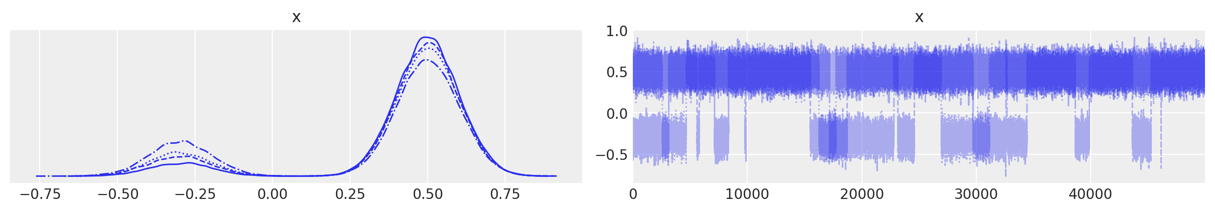
Great. First having a trace we can create Empirical approx
print(pm.Empirical.__doc__)
**Single Group Full Rank Approximation**

    Builds Approximation instance from a given trace,
    it has the same interface as variational approximation
with model:
    approx = pm.Empirical(trace)
approx
<pymc.variational.approximations.Empirical at 0x7f64b15d15b0>
This type of approximation has it’s own underlying storage for samples that is pytensor.shared itself
approx.histogram
histogram
approx.histogram.get_value()[:10]
array([[-0.27366748],
       [-0.32806332],
       [-0.56953621],
       [-0.2994719 ],
       [-0.18962334],
       [-0.24262214],
       [-0.36759098],
       [-0.23522732],
       [-0.37741766],
       [-0.3298074 ]])
approx.histogram.get_value().shape
(200000, 1)
It has exactly the same number of samples that you had in trace before. In our particular case it is 50k. Another thing to notice is that if you have multitrace with more than one chain you’ll get much more samples stored at once. We flatten all the trace for creating Empirical.
This histogram is about how we store samples. The structure is pretty simple: (n_samples, n_dim) The order of these variables is stored internally in the class and in most cases will not be needed for end user
approx.ordering
OrderedDict([('x', ('x', slice(0, 1, None), (), dtype('float64')))])
Sampling from posterior is done uniformly with replacements. Call approx.sample(1000) and you’ll get again the trace but the order is not determined. There is no way now to reconstruct the underlying trace again with approx.sample.
new_trace = approx.sample(50000)
After sampling function is compiled sampling bacomes really fast
az.plot_trace(new_trace);
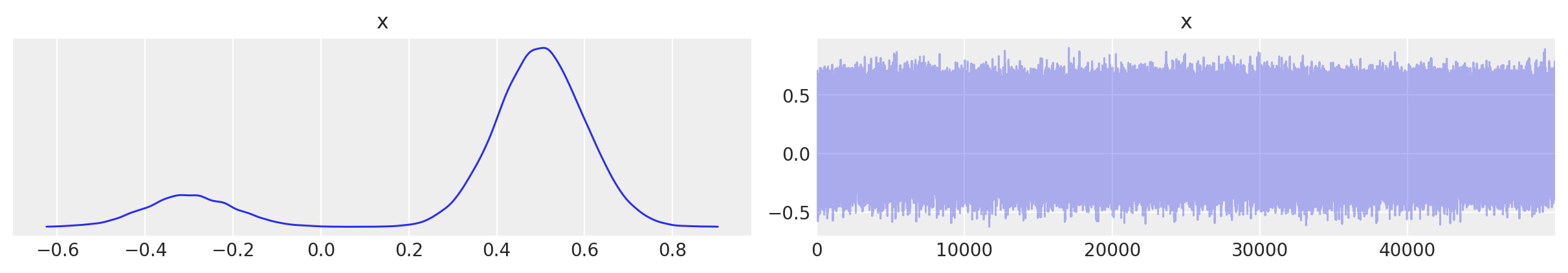
You see there is no order any more but reconstructed density is the same.
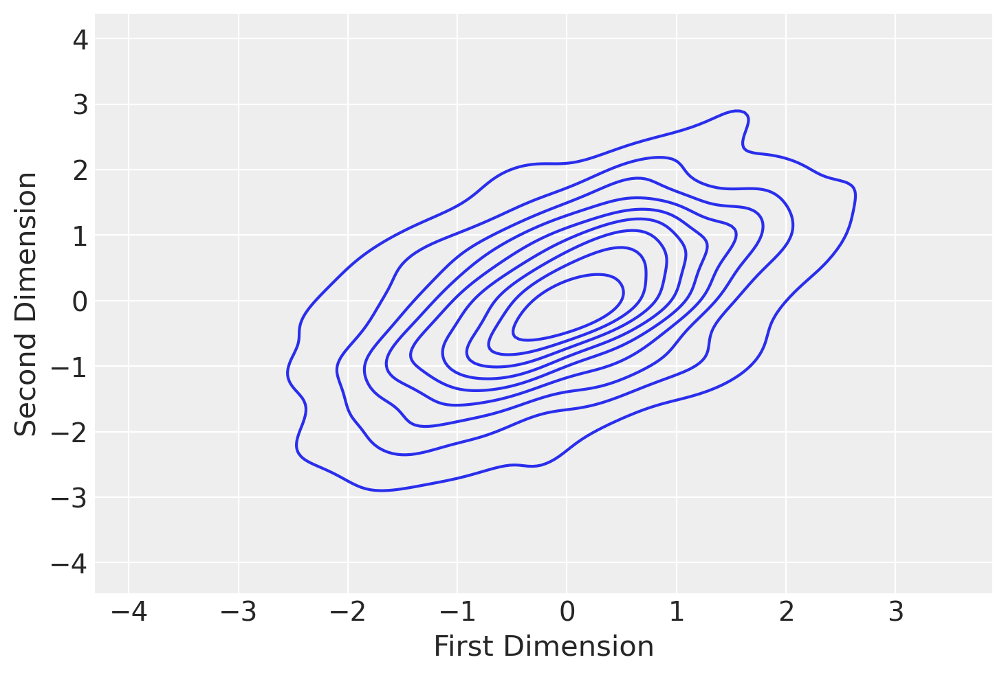
2d density#
mu = pm.floatX([0.0, 0.0])
cov = pm.floatX([[1, 0.5], [0.5, 1.0]])
with pm.Model() as model:
    pm.MvNormal("x", mu=mu, cov=cov, shape=2)
    trace = pm.sample(1000, return_inferencedata=False)
    idata = pm.to_inference_data(trace)
Auto-assigning NUTS sampler...
Initializing NUTS using jitter+adapt_diag...
Multiprocess sampling (4 chains in 4 jobs)
NUTS: [x]
Sampling 4 chains for 1_000 tune and 1_000 draw iterations (4_000 + 4_000 draws total) took 7 seconds.
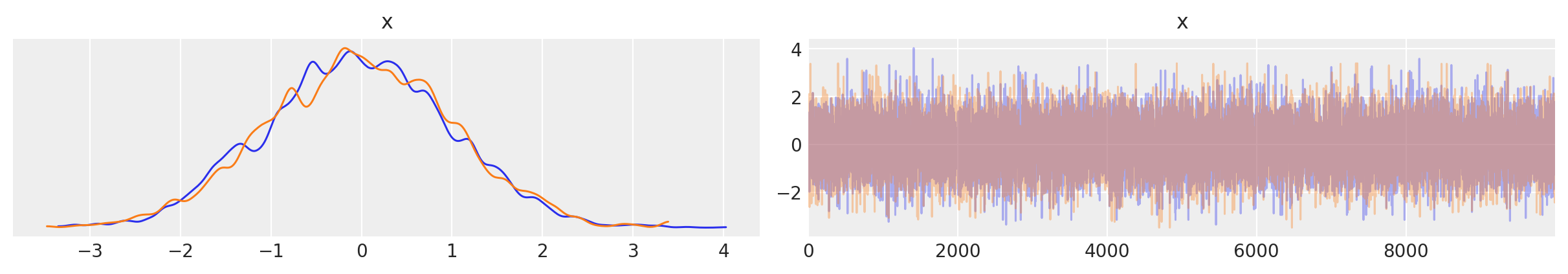
with model:
    approx = pm.Empirical(trace)
az.plot_trace(approx.sample(10000));
Previously we had a trace_cov function
with model:
    print(pm.trace_cov(trace))
[[1.04134257 0.53158646]
 [0.53158646 1.02179671]]
Now we can estimate the same covariance using Empirical
print(approx.cov)
Elemwise{true_div,no_inplace}.0
That’s a tensor object, which we need to evaluate.
print(approx.cov.eval())
[[1.04108223 0.53145356]
 [0.53145356 1.02154126]]
Estimations are very close and differ due to precision error. We can get the mean in the same way
print(approx.mean.eval())
[-0.03548692 -0.03420244]
Watermark#
%load_ext watermark
%watermark -n -u -v -iv -w
Last updated: Fri Jan 13 2023

Python implementation: CPython
Python version       : 3.9.0
IPython version      : 8.8.0

pymc      : 5.0.1
pytensor  : 2.8.11
arviz     : 0.14.0
sys       : 3.9.0 | packaged by conda-forge | (default, Nov 26 2020, 07:57:39)
[GCC 9.3.0]
numpy     : 1.23.5
seaborn   : 0.12.2
matplotlib: 3.6.2

Watermark: 2.3.1
License notice#
All the notebooks in this example gallery are provided under the MIT License which allows modification, and redistribution for any use provided the copyright and license notices are preserved.
Citing PyMC examples#
To cite this notebook, use the DOI provided by Zenodo for the pymc-examples repository.
Important
Many notebooks are adapted from other sources: blogs, books… In such cases you should cite the original source as well.
Also remember to cite the relevant libraries used by your code.
Here is an citation template in bibtex:
@incollection{citekey,
  author    = "<notebook authors, see above>",
  title     = "<notebook title>",
  editor    = "PyMC Team",
  booktitle = "PyMC examples",
  doi       = "10.5281/zenodo.5654871"
}
which once rendered could look like: