Bayesian Vector Autoregressive Models#

import os

import arviz as az
import matplotlib.pyplot as plt
import numpy as np
import pandas as pd
import pymc as pm
import statsmodels.api as sm

from pymc.sampling_jax import sample_blackjax_nuts

/Users/nathanielforde/mambaforge/envs/myjlabenv/lib/python3.11/site-packages/pymc/sampling/jax.py:39: UserWarning: This module is experimental.
  warnings.warn("This module is experimental.")

RANDOM_SEED = 8927
rng = np.random.default_rng(RANDOM_SEED)
az.style.use("arviz-darkgrid")
%config InlineBackend.figure_format = 'retina'

V(ector)A(uto)R(egression) Models#

In this notebook we will outline an application of the Bayesian Vector Autoregressive Modelling. We will draw on the work in the PYMC Labs blogpost (see Vieira [n.d.]). This will be a three part series. In the first we want to show how to fit Bayesian VAR models in PYMC. In the second we will show how to extract extra insight from the fitted model with Impulse Response analysis and make forecasts from the fitted VAR model. In the third and final post we will show in some more detail the benefits of using hierarchical priors with Bayesian VAR models. Specifically, we’ll outline how and why there are actually a range of carefully formulated industry standard priors which work with Bayesian VAR modelling.

In this post we will (i) demonstrate the basic pattern on a simple VAR model on fake data and show how the model recovers the true data generating parameters and (ii) we will show an example applied to macro-economic data and compare the results to those achieved on the same data with statsmodels MLE fits and (iii) show an example of estimating a hierarchical bayesian VAR model over a number of countries.

Autoregressive Models in General#

The idea of a simple autoregressive model is to capture the manner in which past observations of the timeseries are predictive of the current observation. So in traditional fashion, if we model this as a linear phenomena we get simple autoregressive models where the current value is predicted by a weighted linear combination of the past values and an error term.

\[ y_t = \alpha + \beta_{y0} \cdot y_{t-1} + \beta_{y1} \cdot y_{t-2} ... + \epsilon \]

for however many lags are deemed appropriate to the predict the current observation.

A VAR model is kind of generalisation of this framework in that it retains the linear combination approach but allows us to model multiple timeseries at once. So concretely this mean that \(\mathbf{y}_{t}\) as a vector where:

\[ \mathbf{y}_{T} = \nu + A_{1}\mathbf{y}_{T-1} + A_{2}\mathbf{y}_{T-2} ... A_{p}\mathbf{y}_{T-p} + \mathbf{e}_{t} \]

where the As are coefficient matrices to be combined with the past values of each individual timeseries. For example consider an economic example where we aim to model the relationship and mutual influence of each variable on themselves and one another.

\[\begin{split} \begin{bmatrix} gdp \\ inv \\ con \end{bmatrix}_{T} = \nu + A_{1}\begin{bmatrix} gdp \\ inv \\ con \end{bmatrix}_{T-1} + A_{2}\begin{bmatrix} gdp \\ inv \\ con \end{bmatrix}_{T-2} ... A_{p}\begin{bmatrix} gdp \\ inv \\ con \end{bmatrix}_{T-p} + \mathbf{e}_{t} \end{split}\]

This structure is compact representation using matrix notation. The thing we are trying to estimate when we fit a VAR model is the A matrices that determine the nature of the linear combination that best fits our timeseries data. Such timeseries models can have an auto-regressive or a moving average representation, and the details matter for some of the implication of a VAR model fit.

We’ll see in the next notebook of the series how the moving-average representation of a VAR lends itself to the interpretation of the covariance structure in our model as representing a kind of impulse-response relationship between the component timeseries.

A Concrete Specification with Two lagged Terms#

The matrix notation is convenient to suggest the broad patterns of the model, but it is useful to see the algebra is a simple case. Consider the case of Ireland’s GDP and consumption described as:

\[ gdp_{t} = \beta_{gdp1} \cdot gdp_{t-1} + \beta_{gdp2} \cdot gdp_{t-2} + \beta_{cons1} \cdot cons_{t-1} + \beta_{cons2} \cdot cons_{t-2} + \epsilon_{gdp}\]

\[ cons_{t} = \beta_{cons1} \cdot cons_{t-1} + \beta_{cons2} \cdot cons_{t-2} + \beta_{gdp1} \cdot gdp_{t-1} + \beta_{gdp2} \cdot gdp_{t-2} + \epsilon_{cons}\]

In this way we can see that if we can estimate the \(\beta\) terms we have an estimate for the bi-directional effects of each variable on the other. This is a useful feature of the modelling. In what follows i should stress that i’m not an economist and I’m aiming to show only the functionality of these models not give you a decisive opinion about the economic relationships determining Irish GDP figures.

Creating some Fake Data#

def simulate_var(
    intercepts, coefs_yy, coefs_xy, coefs_xx, coefs_yx, noises=(1, 1), *, warmup=100, steps=200
):
    draws_y = np.zeros(warmup + steps)
    draws_x = np.zeros(warmup + steps)
    draws_y[:2] = intercepts[0]
    draws_x[:2] = intercepts[1]
    for step in range(2, warmup + steps):
        draws_y[step] = (
            intercepts[0]
            + coefs_yy[0] * draws_y[step - 1]
            + coefs_yy[1] * draws_y[step - 2]
            + coefs_xy[0] * draws_x[step - 1]
            + coefs_xy[1] * draws_x[step - 2]
            + rng.normal(0, noises[0])
        )
        draws_x[step] = (
            intercepts[1]
            + coefs_xx[0] * draws_x[step - 1]
            + coefs_xx[1] * draws_x[step - 2]
            + coefs_yx[0] * draws_y[step - 1]
            + coefs_yx[1] * draws_y[step - 2]
            + rng.normal(0, noises[1])
        )
    return draws_y[warmup:], draws_x[warmup:]

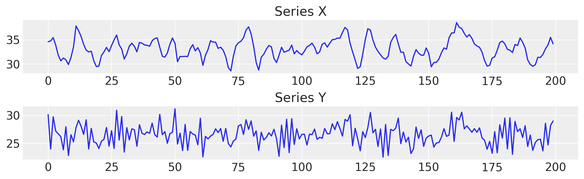
First we generate some fake data with known parameters.

var_y, var_x = simulate_var(
    intercepts=(18, 8),
    coefs_yy=(-0.8, 0),
    coefs_xy=(0.9, 0),
    coefs_xx=(1.3, -0.7),
    coefs_yx=(-0.1, 0.3),
)

df = pd.DataFrame({"x": var_x, "y": var_y})
df.head()

	x	y
0	34.606613	30.117581
1	34.773803	23.996700
2	35.455237	29.738941
3	33.886706	27.193417
4	31.837465	26.704728

fig, axs = plt.subplots(2, 1, figsize=(10, 3))
axs[0].plot(df["x"], label="x")
axs[0].set_title("Series X")
axs[1].plot(df["y"], label="y")
axs[1].set_title("Series Y");

../_images/ecc3bd5333e15cb66600373124e070d5a3e3bc9eeaf273614597721ef6ea9aa9.png

Handling Multiple Lags and Different Dimensions#

When Modelling multiple timeseries and accounting for potentially any number lags to incorporate in our model we need to abstract some of the model definition to helper functions. An example will make this a bit clearer.

### Define a helper function that will construct our autoregressive step for the marginal contribution of each lagged
### term in each of the respective time series equations
def calc_ar_step(lag_coefs, n_eqs, n_lags, df):
    ars = []
    for j in range(n_eqs):
        ar = pm.math.sum(
            [
                pm.math.sum(lag_coefs[j, i] * df.values[n_lags - (i + 1) : -(i + 1)], axis=-1)
                for i in range(n_lags)
            ],
            axis=0,
        )
        ars.append(ar)
    beta = pm.math.stack(ars, axis=-1)

    return beta


### Make the model in such a way that it can handle different specifications of the likelihood term
### and can be run for simple prior predictive checks. This latter functionality is important for debugging of
### shape handling issues. Building a VAR model involves quite a few moving parts and it is handy to
### inspect the shape implied in the prior predictive checks.
def make_model(n_lags, n_eqs, df, priors, mv_norm=True, prior_checks=True):
    coords = {
        "lags": np.arange(n_lags) + 1,
        "equations": df.columns.tolist(),
        "cross_vars": df.columns.tolist(),
        "time": [x for x in df.index[n_lags:]],
    }

    with pm.Model(coords=coords) as model:
        lag_coefs = pm.Normal(
            "lag_coefs",
            mu=priors["lag_coefs"]["mu"],
            sigma=priors["lag_coefs"]["sigma"],
            dims=["equations", "lags", "cross_vars"],
        )
        alpha = pm.Normal(
            "alpha", mu=priors["alpha"]["mu"], sigma=priors["alpha"]["sigma"], dims=("equations",)
        )
        data_obs = pm.Data("data_obs", df.values[n_lags:], dims=["time", "equations"], mutable=True)

        betaX = calc_ar_step(lag_coefs, n_eqs, n_lags, df)
        betaX = pm.Deterministic(
            "betaX",
            betaX,
            dims=[
                "time",
            ],
        )
        mean = alpha + betaX

        if mv_norm:
            n = df.shape[1]
            ## Under the hood the LKJ prior will retain the correlation matrix too.
            noise_chol, _, _ = pm.LKJCholeskyCov(
                "noise_chol",
                eta=priors["noise_chol"]["eta"],
                n=n,
                sd_dist=pm.HalfNormal.dist(sigma=priors["noise_chol"]["sigma"]),
            )
            obs = pm.MvNormal(
                "obs", mu=mean, chol=noise_chol, observed=data_obs, dims=["time", "equations"]
            )
        else:
            ## This is an alternative likelihood that can recover sensible estimates of the coefficients
            ## But lacks the multivariate correlation between the timeseries.
            sigma = pm.HalfNormal("noise", sigma=priors["noise"]["sigma"], dims=["equations"])
            obs = pm.Normal(
                "obs", mu=mean, sigma=sigma, observed=data_obs, dims=["time", "equations"]
            )

        if prior_checks:
            idata = pm.sample_prior_predictive()
            return model, idata
        else:
            idata = pm.sample_prior_predictive()
            idata.extend(pm.sample(draws=2000, random_seed=130))
            pm.sample_posterior_predictive(idata, extend_inferencedata=True, random_seed=rng)
    return model, idata

The model has a deterministic component in the auto-regressive calculation which is required at each timestep, but the key point here is that we model the likelihood of the VAR as a multivariate normal distribution with a particular covariance relationship. The estimation of these covariance relationship gives the main insight in the manner in which our component timeseries relate to one another.

We will inspect the structure of a VAR with 2 lags and 2 equations

n_lags = 2
n_eqs = 2
priors = {
    "lag_coefs": {"mu": 0.3, "sigma": 1},
    "alpha": {"mu": 15, "sigma": 5},
    "noise_chol": {"eta": 1, "sigma": 1},
    "noise": {"sigma": 1},
}

model, idata = make_model(n_lags, n_eqs, df, priors)
pm.model_to_graphviz(model)

Sampling: [alpha, lag_coefs, noise_chol, obs]

../_images/46db3979a328b9ac4ca045fdf34c75b2eb372ec81c2aa8d06daddab5b61b7c29.svg

Another VAR with 3 lags and 2 equations.

n_lags = 3
n_eqs = 2
model, idata = make_model(n_lags, n_eqs, df, priors)
for rv, shape in model.eval_rv_shapes().items():
    print(f"{rv:>11}: shape={shape}")
pm.model_to_graphviz(model)

Sampling: [alpha, lag_coefs, noise_chol, obs]

  lag_coefs: shape=(2, 3, 2)
      alpha: shape=(2,)
noise_chol_cholesky-cov-packed__: shape=(3,)
 noise_chol: shape=(3,)

../_images/b0e658b7e9bee038b23b6d2680e8c0554015e9c3dce1186a5f8db9caf47ea709.svg

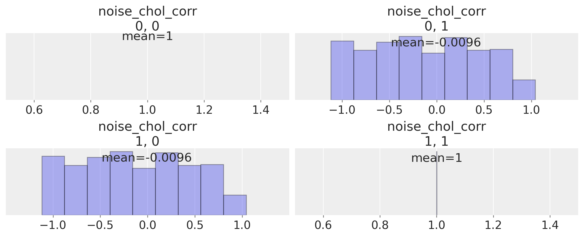
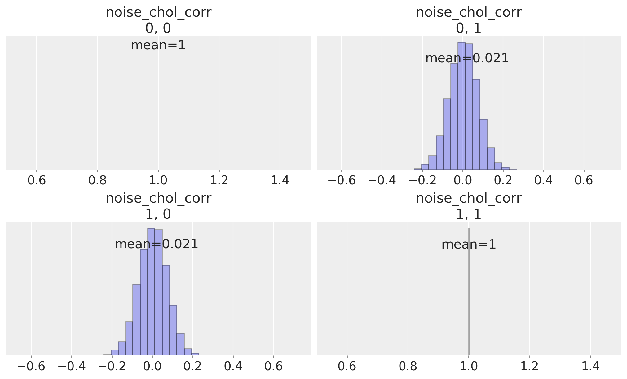
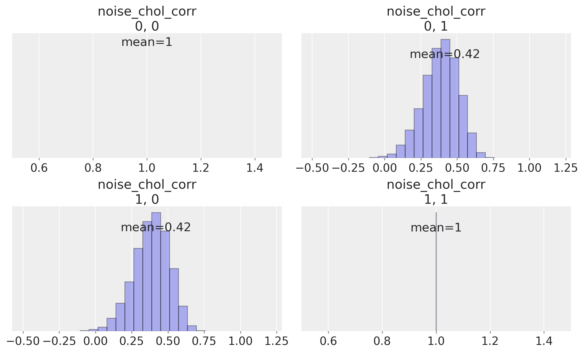
We can inspect the correlation matrix between our timeseries which is implied by the prior specification, to see that we have allowed a flat uniform prior over their correlation.

ax = az.plot_posterior(
    idata,
    var_names="noise_chol_corr",
    hdi_prob="hide",
    group="prior",
    point_estimate="mean",
    grid=(2, 2),
    kind="hist",
    ec="black",
    figsize=(10, 4),
)

../_images/30e5645b049e2276555bfba26d9640e5499c83d2824f9614e964ddf5c6f2b6cf.png

Now we will fit the VAR with 2 lags and 2 equations

n_lags = 2
n_eqs = 2
model, idata_fake_data = make_model(n_lags, n_eqs, df, priors, prior_checks=False)

Sampling: [alpha, lag_coefs, noise_chol, obs]
Auto-assigning NUTS sampler...
Initializing NUTS using jitter+adapt_diag...
Multiprocess sampling (4 chains in 4 jobs)
NUTS: [lag_coefs, alpha, noise_chol]

100.00% [12000/12000 05:59<00:00 Sampling 4 chains, 0 divergences]

Sampling 4 chains for 1_000 tune and 2_000 draw iterations (4_000 + 8_000 draws total) took 360 seconds.
Sampling: [obs]

100.00% [8000/8000 02:11<00:00]

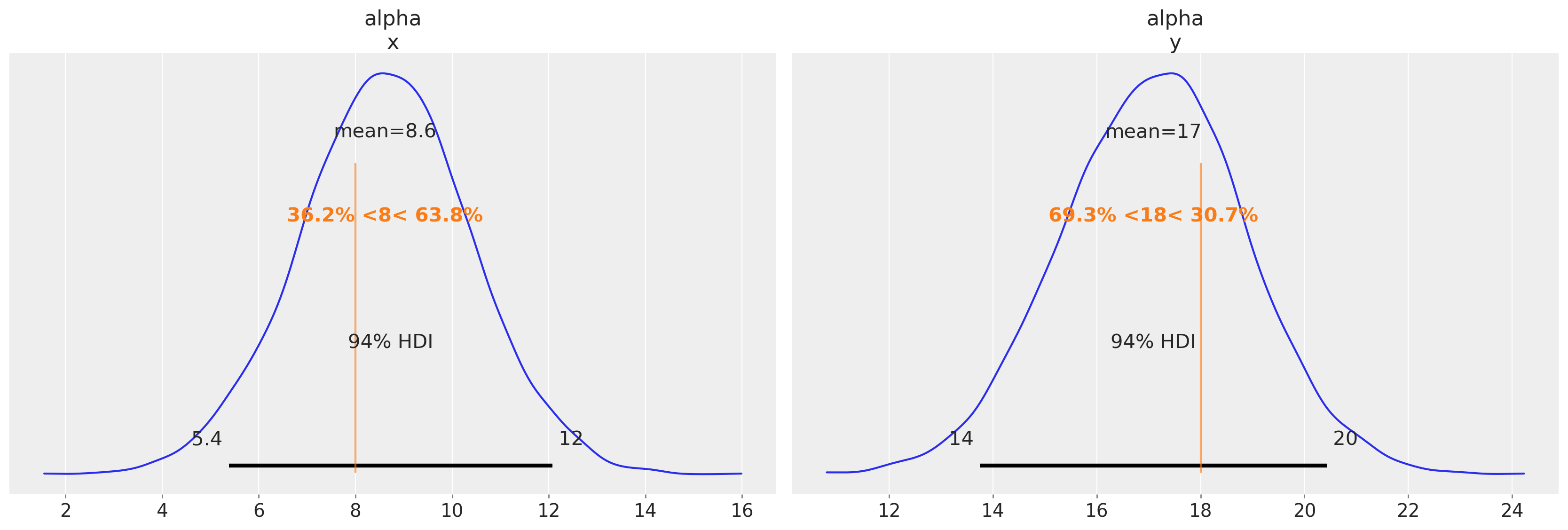
We’ll now plot some of the results to see that the parameters are being broadly recovered. The alpha parameters match well, but the individual lag coefficients show differences.

az.summary(idata_fake_data, var_names=["alpha", "lag_coefs", "noise_chol_corr"])

/Users/nathanielforde/mambaforge/envs/myjlabenv/lib/python3.11/site-packages/arviz/stats/diagnostics.py:584: RuntimeWarning: invalid value encountered in scalar divide
  (between_chain_variance / within_chain_variance + num_samples - 1) / (num_samples)

	mean	sd	hdi_3%	hdi_97%	mcse_mean	mcse_sd	ess_bulk	ess_tail	r_hat
alpha[x]	8.607	1.765	5.380	12.076	0.029	0.020	3823.0	4602.0	1.0
alpha[y]	17.094	1.778	13.750	20.431	0.027	0.019	4188.0	5182.0	1.0
lag_coefs[x, 1, x]	1.333	0.062	1.218	1.450	0.001	0.001	5564.0	4850.0	1.0
lag_coefs[x, 1, y]	-0.120	0.069	-0.247	0.011	0.001	0.001	3739.0	4503.0	1.0
lag_coefs[x, 2, x]	-0.711	0.097	-0.890	-0.527	0.002	0.001	3629.0	4312.0	1.0
lag_coefs[x, 2, y]	0.267	0.073	0.126	0.403	0.001	0.001	3408.0	4318.0	1.0
lag_coefs[y, 1, x]	0.838	0.061	0.718	0.948	0.001	0.001	5203.0	5345.0	1.0
lag_coefs[y, 1, y]	-0.800	0.069	-0.932	-0.673	0.001	0.001	3749.0	5131.0	1.0
lag_coefs[y, 2, x]	0.094	0.097	-0.087	0.277	0.002	0.001	3573.0	4564.0	1.0
lag_coefs[y, 2, y]	-0.004	0.074	-0.145	0.133	0.001	0.001	3448.0	4484.0	1.0
noise_chol_corr[0, 0]	1.000	0.000	1.000	1.000	0.000	0.000	8000.0	8000.0	NaN
noise_chol_corr[0, 1]	0.021	0.072	-0.118	0.152	0.001	0.001	6826.0	5061.0	1.0
noise_chol_corr[1, 0]	0.021	0.072	-0.118	0.152	0.001	0.001	6826.0	5061.0	1.0
noise_chol_corr[1, 1]	1.000	0.000	1.000	1.000	0.000	0.000	7813.0	7824.0	1.0

az.plot_posterior(idata_fake_data, var_names=["alpha"], ref_val=[8, 18]);

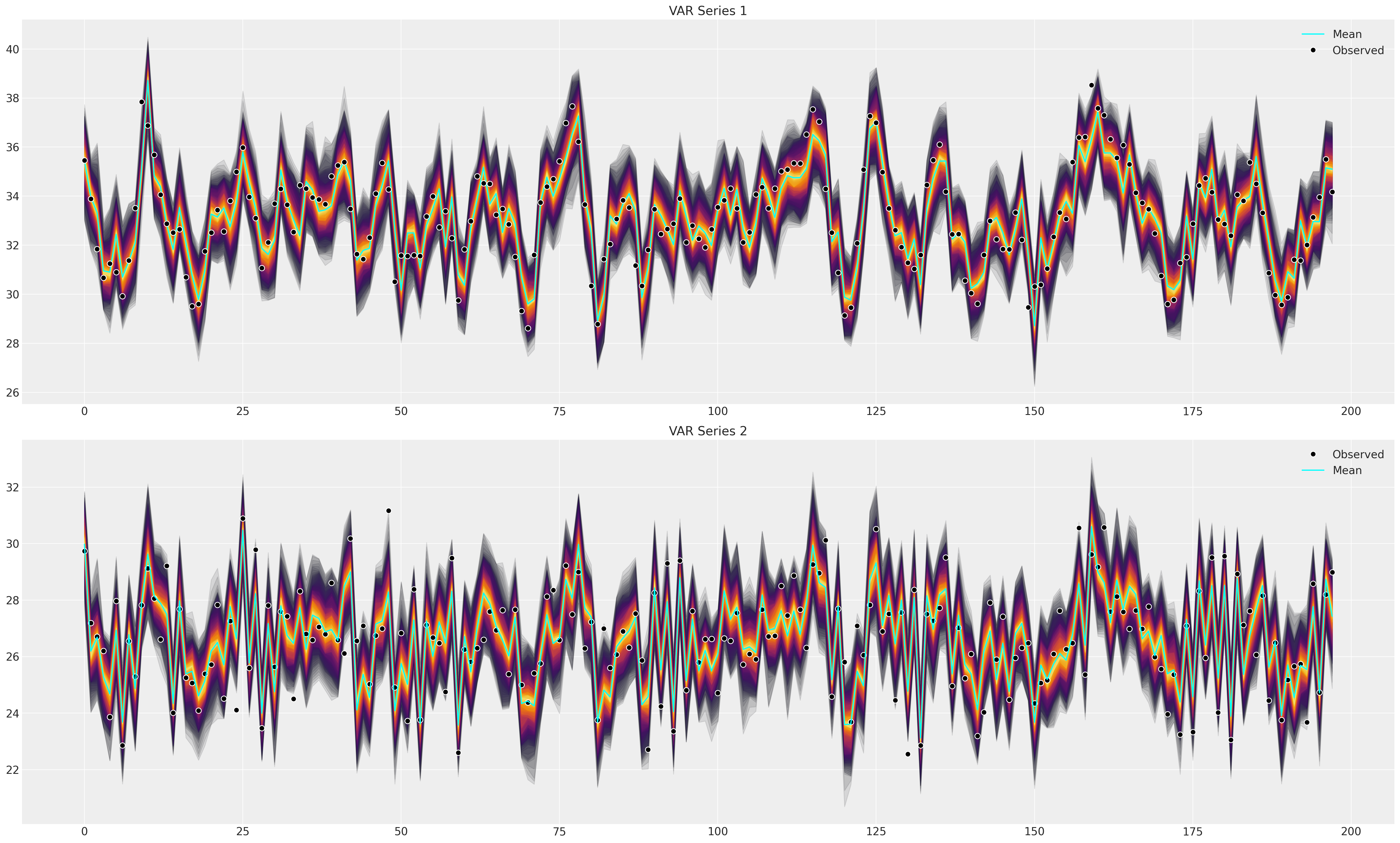
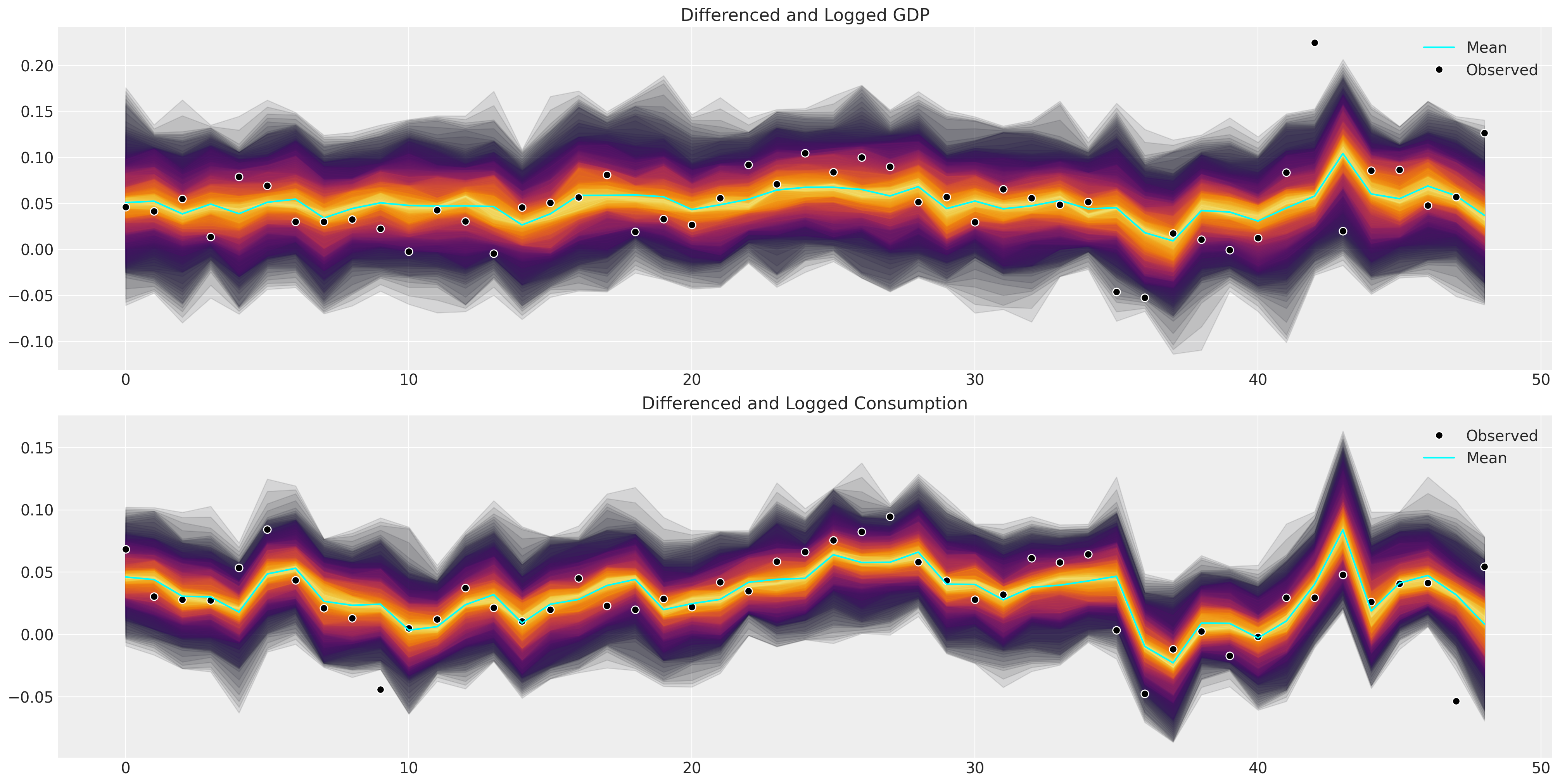
../_images/4d7eb64f5ff15a8229c61d0b7226c784c23a4180382b2c37079f45a01dbfe5c0.png

Next we’ll plot the posterior predictive distribution to check that the fitted model can capture the patterns in the observed data. This is the primary test of goodness of fit.

def shade_background(ppc, ax, idx, palette="cividis"):
    palette = palette
    cmap = plt.get_cmap(palette)
    percs = np.linspace(51, 99, 100)
    colors = (percs - np.min(percs)) / (np.max(percs) - np.min(percs))
    for i, p in enumerate(percs[::-1]):
        upper = np.percentile(
            ppc[:, idx, :],
            p,
            axis=1,
        )
        lower = np.percentile(
            ppc[:, idx, :],
            100 - p,
            axis=1,
        )
        color_val = colors[i]
        ax[idx].fill_between(
            x=np.arange(ppc.shape[0]),
            y1=upper.flatten(),
            y2=lower.flatten(),
            color=cmap(color_val),
            alpha=0.1,
        )


def plot_ppc(idata, df, group="posterior_predictive"):
    fig, axs = plt.subplots(2, 1, figsize=(25, 15))
    df = pd.DataFrame(idata_fake_data["observed_data"]["obs"].data, columns=["x", "y"])
    axs = axs.flatten()
    ppc = az.extract(idata, group=group, num_samples=100)["obs"]
    # Minus the lagged terms and the constant
    shade_background(ppc, axs, 0, "inferno")
    axs[0].plot(np.arange(ppc.shape[0]), ppc[:, 0, :].mean(axis=1), color="cyan", label="Mean")
    axs[0].plot(df["x"], "o", mfc="black", mec="white", mew=1, markersize=7, label="Observed")
    axs[0].set_title("VAR Series 1")
    axs[0].legend()
    shade_background(ppc, axs, 1, "inferno")
    axs[1].plot(df["y"], "o", mfc="black", mec="white", mew=1, markersize=7, label="Observed")
    axs[1].plot(np.arange(ppc.shape[0]), ppc[:, 1, :].mean(axis=1), color="cyan", label="Mean")
    axs[1].set_title("VAR Series 2")
    axs[1].legend()


plot_ppc(idata_fake_data, df)

../_images/4cc2d4d22fd292017c1b8597b2f9e23929a0a13ed2936b03e14f9038c40ccd84.png

Again we can check the learned posterior distribution for the correlation parameter.

ax = az.plot_posterior(
    idata_fake_data,
    var_names="noise_chol_corr",
    hdi_prob="hide",
    point_estimate="mean",
    grid=(2, 2),
    kind="hist",
    ec="black",
    figsize=(10, 6),
)

../_images/4ba85f65960464ed574fbf89fe8162e4faade29acef50963c3c62b6cd7d49f0d.png

Applying the Theory: Macro Economic Timeseries#

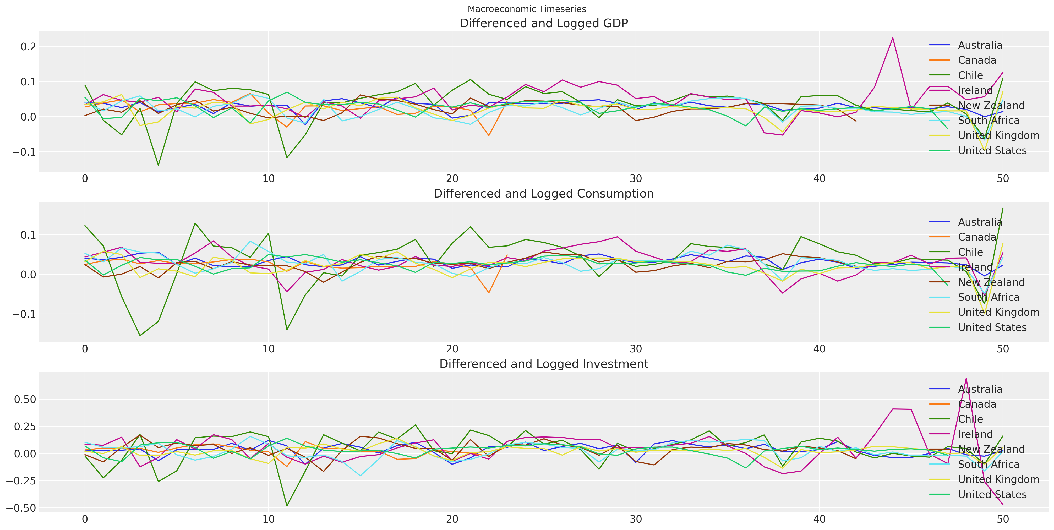
The data is from the World Bank’s World Development Indicators. In particular, we’re pulling annual values of GDP, consumption, and gross fixed capital formation (investment) for all countries from 1970. Timeseries models in general work best when we have a stable mean throughout the series, so for the estimation procedure we have taken the first difference and the natural log of each of these series.

try:
    gdp_hierarchical = pd.read_csv(
        os.path.join("..", "data", "gdp_data_hierarchical_clean.csv"), index_col=0
    )
except FileNotFoundError:
    gdp_hierarchical = pd.read_csv(pm.get_data("gdp_data_hierarchical_clean.csv"), ...)

gdp_hierarchical

	country	iso2c	iso3c	year	GDP	CONS	GFCF	dl_gdp	dl_cons	dl_gfcf	more_than_10	time
1	Australia	AU	AUS	1971	4.647670e+11	3.113170e+11	7.985100e+10	0.039217	0.040606	0.031705	True	1
2	Australia	AU	AUS	1972	4.829350e+11	3.229650e+11	8.209200e+10	0.038346	0.036732	0.027678	True	2
3	Australia	AU	AUS	1973	4.955840e+11	3.371070e+11	8.460300e+10	0.025855	0.042856	0.030129	True	3
4	Australia	AU	AUS	1974	5.159300e+11	3.556010e+11	8.821400e+10	0.040234	0.053409	0.041796	True	4
5	Australia	AU	AUS	1975	5.228210e+11	3.759000e+11	8.255900e+10	0.013268	0.055514	-0.066252	True	5
...	...	...	...	...	...	...	...	...	...	...	...	...
366	United States	US	USA	2016	1.850960e+13	1.522497e+13	3.802207e+12	0.016537	0.023425	0.021058	True	44
367	United States	US	USA	2017	1.892712e+13	1.553075e+13	3.947418e+12	0.022306	0.019885	0.037480	True	45
368	United States	US	USA	2018	1.947957e+13	1.593427e+13	4.119951e+12	0.028771	0.025650	0.042780	True	46
369	United States	US	USA	2019	1.992544e+13	1.627888e+13	4.248643e+12	0.022631	0.021396	0.030758	True	47
370	United States	US	USA	2020	1.924706e+13	1.582501e+13	4.182801e+12	-0.034639	-0.028277	-0.015619	True	48

370 rows × 12 columns

fig, axs = plt.subplots(3, 1, figsize=(20, 10))
for country in gdp_hierarchical["country"].unique():
    temp = gdp_hierarchical[gdp_hierarchical["country"] == country].reset_index()
    axs[0].plot(temp["dl_gdp"], label=f"{country}")
    axs[1].plot(temp["dl_cons"], label=f"{country}")
    axs[2].plot(temp["dl_gfcf"], label=f"{country}")
axs[0].set_title("Differenced and Logged GDP")
axs[1].set_title("Differenced and Logged Consumption")
axs[2].set_title("Differenced and Logged Investment")
axs[0].legend()
axs[1].legend()
axs[2].legend()
plt.suptitle("Macroeconomic Timeseries");

../_images/4e2642a8e46e880c72e474b3db11d9728e98dc58908f61da9d28e92bee721052.png

Ireland’s Economic Situation#

Ireland is somewhat infamous for its GDP numbers that are largely the product of foreign direct investment and inflated beyond expectation in recent years by the investment and taxation deals offered to large multi-nationals. We’ll look here at just the relationship between GDP and consumption. We just want to show the mechanics of the VAR estimation, you shouldn’t read too much into the subsequent analysis.

ireland_df = gdp_hierarchical[gdp_hierarchical["country"] == "Ireland"]
ireland_df.reset_index(inplace=True, drop=True)
ireland_df.head()

	country	iso2c	iso3c	year	GDP	CONS	GFCF	dl_gdp	dl_cons	dl_gfcf	more_than_10	time
0	Ireland	IE	IRL	1971	3.314234e+10	2.897699e+10	8.317518e+09	0.034110	0.043898	0.085452	True	1
1	Ireland	IE	IRL	1972	3.529322e+10	3.063538e+10	8.967782e+09	0.062879	0.055654	0.075274	True	2
2	Ireland	IE	IRL	1973	3.695956e+10	3.280221e+10	1.041728e+10	0.046134	0.068340	0.149828	True	3
3	Ireland	IE	IRL	1974	3.853412e+10	3.381524e+10	9.207243e+09	0.041720	0.030416	-0.123476	True	4
4	Ireland	IE	IRL	1975	4.071386e+10	3.477232e+10	8.874887e+09	0.055024	0.027910	-0.036765	True	5

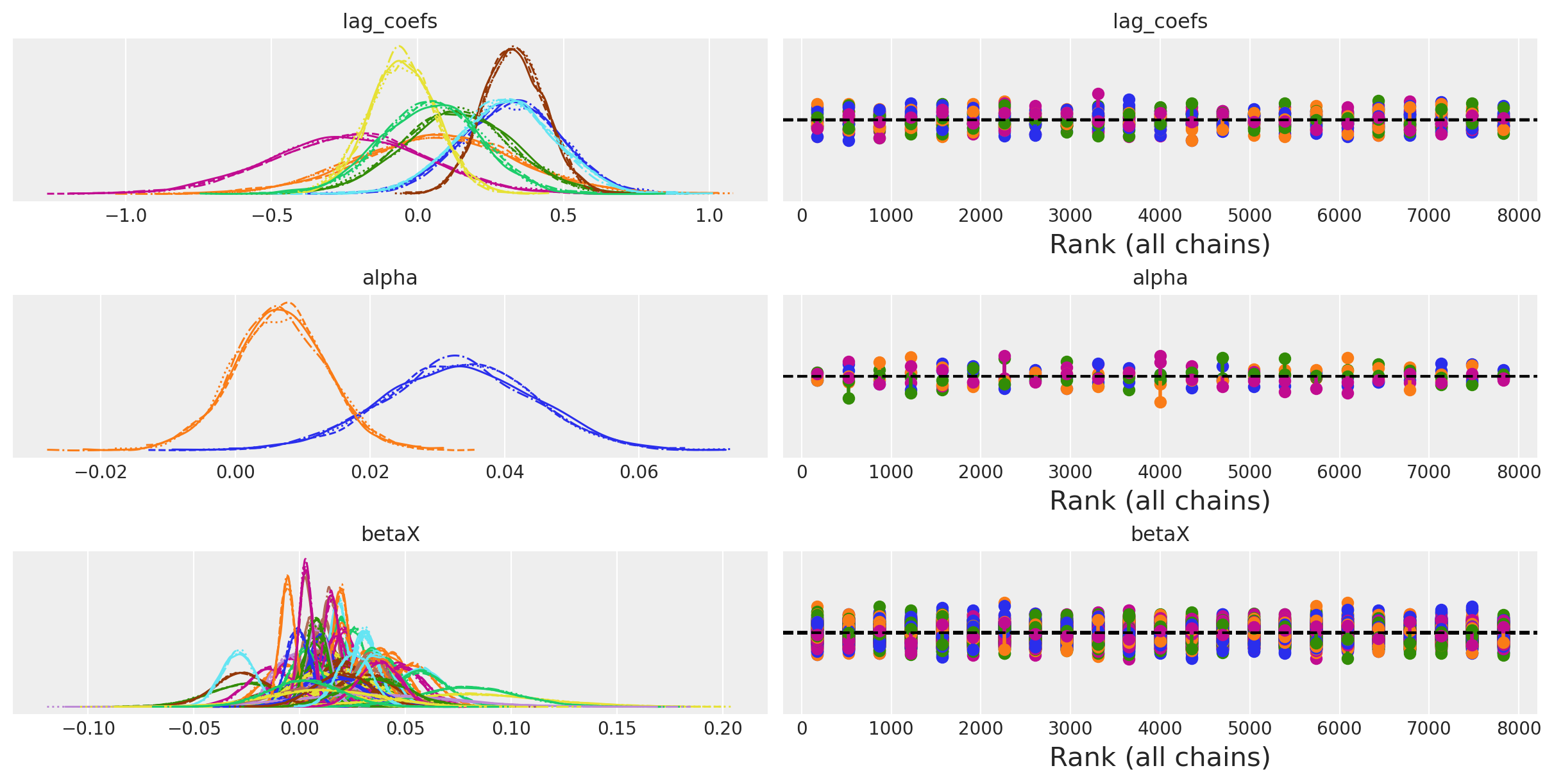
az.plot_trace(idata_ireland, var_names=["lag_coefs", "alpha", "betaX"], kind="rank_vlines");

../_images/063abe8a9272f0339cf7f3d814d8505c716f95d2846242b4017d6f23a605059b.png

def plot_ppc_macro(idata, df, group="posterior_predictive"):
    df = pd.DataFrame(idata["observed_data"]["obs"].data, columns=["dl_gdp", "dl_cons"])
    fig, axs = plt.subplots(2, 1, figsize=(20, 10))
    axs = axs.flatten()
    ppc = az.extract(idata, group=group, num_samples=100)["obs"]

    shade_background(ppc, axs, 0, "inferno")
    axs[0].plot(np.arange(ppc.shape[0]), ppc[:, 0, :].mean(axis=1), color="cyan", label="Mean")
    axs[0].plot(df["dl_gdp"], "o", mfc="black", mec="white", mew=1, markersize=7, label="Observed")
    axs[0].set_title("Differenced and Logged GDP")
    axs[0].legend()
    shade_background(ppc, axs, 1, "inferno")
    axs[1].plot(df["dl_cons"], "o", mfc="black", mec="white", mew=1, markersize=7, label="Observed")
    axs[1].plot(np.arange(ppc.shape[0]), ppc[:, 1, :].mean(axis=1), color="cyan", label="Mean")
    axs[1].set_title("Differenced and Logged Consumption")
    axs[1].legend()


plot_ppc_macro(idata_ireland, ireland_df)

../_images/762ce8a1ab002a935bc3005e61db46f73334a5676f781fd91760e1a592adb28a.png

ax = az.plot_posterior(
    idata_ireland,
    var_names="noise_chol_corr",
    hdi_prob="hide",
    point_estimate="mean",
    grid=(2, 2),
    kind="hist",
    ec="black",
    figsize=(10, 6),
)

../_images/85dc433748b1cabd042f50cbea09d5fe9ea6c7cce63f2aabc01fc4c56657f7ba.png

Comparison with Statsmodels#

It’s worthwhile comparing these model fits to the one achieved by Statsmodels just to see if we can recover a similar story.

VAR_model = sm.tsa.VAR(ireland_df[["dl_gdp", "dl_cons"]])
results = VAR_model.fit(2, trend="c")

results.params

	dl_gdp	dl_cons
const	0.034145	0.006996
L1.dl_gdp	0.324904	0.330003
L1.dl_cons	0.076629	0.305824
L2.dl_gdp	0.137721	-0.053677
L2.dl_cons	-0.278745	0.033728

The intercept parameters broadly agree with our Bayesian model with some differences in the implied relationships defined by the estimates for the lagged terms.

corr = pd.DataFrame(results.resid_corr, columns=["dl_gdp", "dl_cons"])
corr.index = ["dl_gdp", "dl_cons"]
corr

	dl_gdp	dl_cons
dl_gdp	1.000000	0.435807
dl_cons	0.435807	1.000000

The residual correlation estimates reported by statsmodels agree quite closely with the multivariate gaussian correlation between the variables in our Bayesian model.

az.summary(idata_ireland, var_names=["alpha", "lag_coefs", "noise_chol_corr"])

/Users/nathanielforde/mambaforge/envs/myjlabenv/lib/python3.11/site-packages/arviz/stats/diagnostics.py:584: RuntimeWarning: invalid value encountered in scalar divide
  (between_chain_variance / within_chain_variance + num_samples - 1) / (num_samples)

	mean	sd	hdi_3%	hdi_97%	mcse_mean	mcse_sd	ess_bulk	ess_tail	r_hat
alpha[dl_gdp]	0.033	0.011	0.012	0.053	0.000	0.000	6683.0	5919.0	1.0
alpha[dl_cons]	0.007	0.007	-0.007	0.020	0.000	0.000	7651.0	5999.0	1.0
lag_coefs[dl_gdp, 1, dl_gdp]	0.321	0.170	0.008	0.642	0.002	0.002	6984.0	6198.0	1.0
lag_coefs[dl_gdp, 1, dl_cons]	0.071	0.273	-0.447	0.582	0.003	0.003	7376.0	5466.0	1.0
lag_coefs[dl_gdp, 2, dl_gdp]	0.133	0.190	-0.228	0.488	0.002	0.002	7471.0	6128.0	1.0
lag_coefs[dl_gdp, 2, dl_cons]	-0.235	0.269	-0.748	0.259	0.003	0.002	8085.0	5963.0	1.0
lag_coefs[dl_cons, 1, dl_gdp]	0.331	0.106	0.133	0.528	0.001	0.001	7670.0	6360.0	1.0
lag_coefs[dl_cons, 1, dl_cons]	0.302	0.170	-0.012	0.616	0.002	0.001	7963.0	6150.0	1.0
lag_coefs[dl_cons, 2, dl_gdp]	-0.054	0.118	-0.279	0.163	0.001	0.001	8427.0	6296.0	1.0
lag_coefs[dl_cons, 2, dl_cons]	0.048	0.170	-0.259	0.378	0.002	0.002	8669.0	6264.0	1.0
noise_chol_corr[0, 0]	1.000	0.000	1.000	1.000	0.000	0.000	8000.0	8000.0	NaN
noise_chol_corr[0, 1]	0.416	0.123	0.180	0.633	0.001	0.001	9155.0	6052.0	1.0
noise_chol_corr[1, 0]	0.416	0.123	0.180	0.633	0.001	0.001	9155.0	6052.0	1.0
noise_chol_corr[1, 1]	1.000	0.000	1.000	1.000	0.000	0.000	7871.0	8000.0	1.0

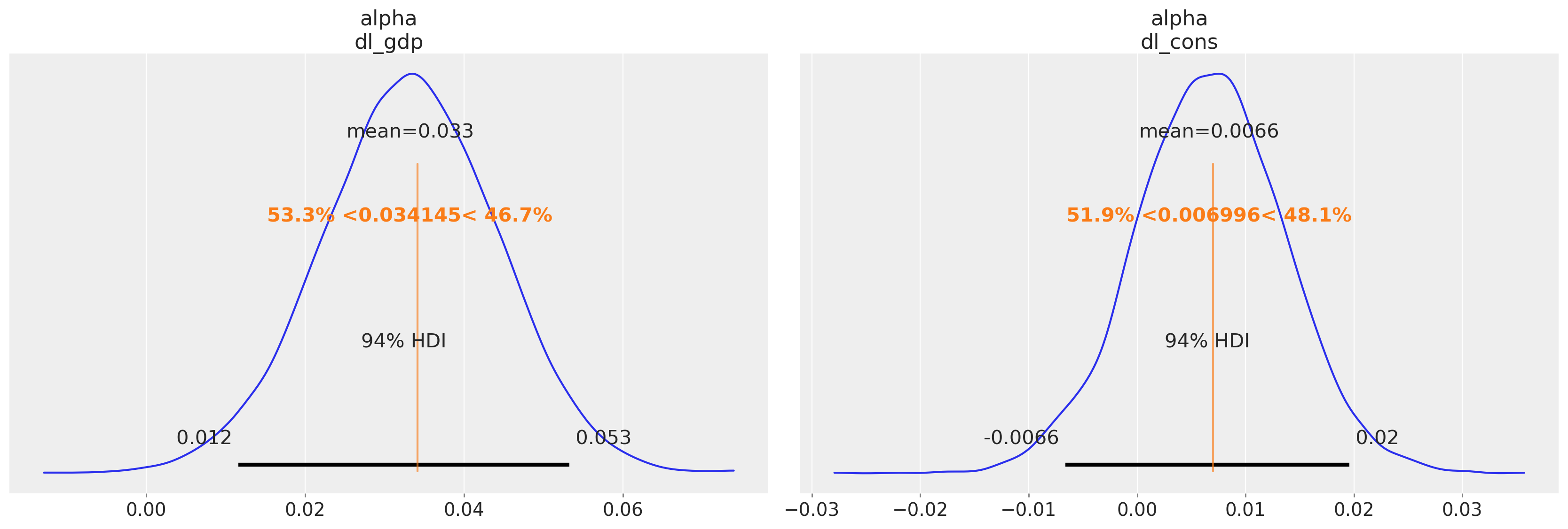
We plot the alpha parameter estimates against the Statsmodels estimates

az.plot_posterior(idata_ireland, var_names=["alpha"], ref_val=[0.034145, 0.006996]);

../_images/bca8db365b5899de2b68e81fd2f6816c9025404bf29b6a61a603314acfef7a33.png

az.plot_posterior(
    idata_ireland,
    var_names=["lag_coefs"],
    ref_val=[0.330003, -0.053677],
    coords={"equations": "dl_cons", "lags": [1, 2], "cross_vars": "dl_gdp"},
);

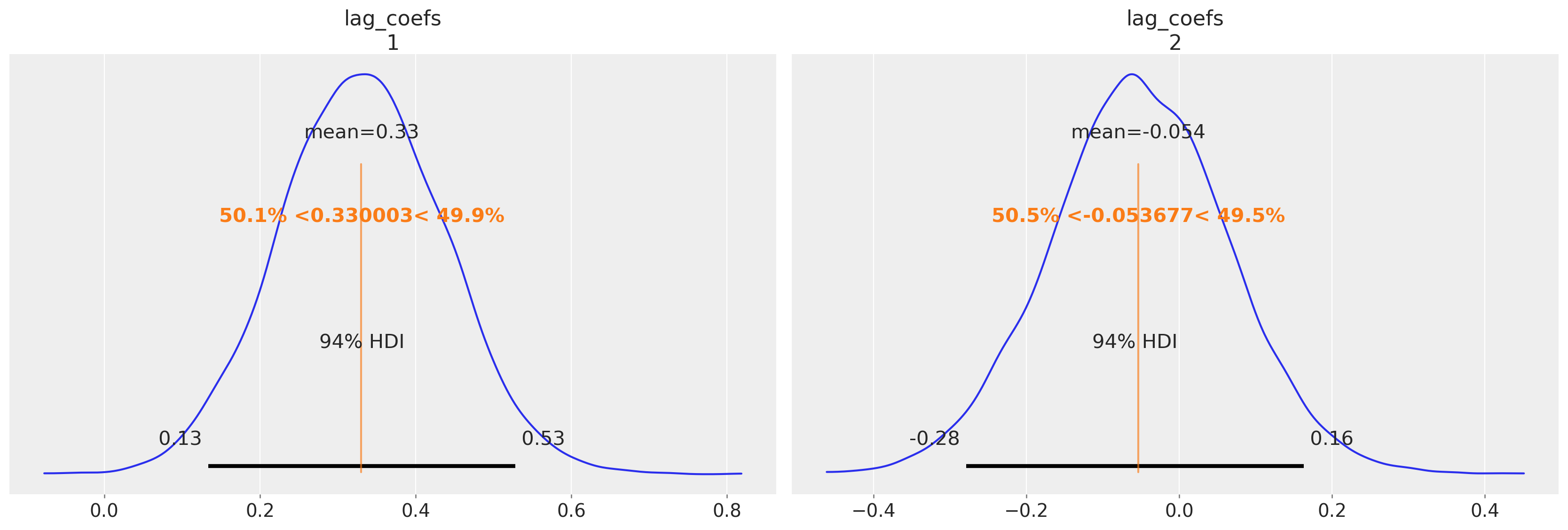
../_images/21fd827e56c649e0d9da4ecfc65752ccc706f5f52b2ef06a1ba352b67cd08968.png

We can see here again how the Bayesian VAR model recovers much of the same story. Similar magnitudes in the estimates for the alpha terms for both equations and a clear relationship between the first lagged GDP numbers and consumption along with a very similar covariance structure.

Adding a Bayesian Twist: Hierarchical VARs#

In addition we can add some hierarchical parameters if we want to model multiple countries and the relationship between these economic metrics at the national level. This is a useful technique in the cases where we have reasonably short timeseries data because it allows us to “borrow” information across the countries to inform the estimates of the key parameters.

def make_hierarchical_model(n_lags, n_eqs, df, group_field, prior_checks=True):
    cols = [col for col in df.columns if col != group_field]
    coords = {"lags": np.arange(n_lags) + 1, "equations": cols, "cross_vars": cols}

    groups = df[group_field].unique()

    with pm.Model(coords=coords) as model:
        ## Hierarchical Priors
        rho = pm.Beta("rho", alpha=2, beta=2)
        alpha_hat_location = pm.Normal("alpha_hat_location", 0, 0.1)
        alpha_hat_scale = pm.InverseGamma("alpha_hat_scale", 3, 0.5)
        beta_hat_location = pm.Normal("beta_hat_location", 0, 0.1)
        beta_hat_scale = pm.InverseGamma("beta_hat_scale", 3, 0.5)
        omega_global, _, _ = pm.LKJCholeskyCov(
            "omega_global", n=n_eqs, eta=1.0, sd_dist=pm.Exponential.dist(1)
        )

        for grp in groups:
            df_grp = df[df[group_field] == grp][cols]
            z_scale_beta = pm.InverseGamma(f"z_scale_beta_{grp}", 3, 0.5)
            z_scale_alpha = pm.InverseGamma(f"z_scale_alpha_{grp}", 3, 0.5)
            lag_coefs = pm.Normal(
                f"lag_coefs_{grp}",
                mu=beta_hat_location,
                sigma=beta_hat_scale * z_scale_beta,
                dims=["equations", "lags", "cross_vars"],
            )
            alpha = pm.Normal(
                f"alpha_{grp}",
                mu=alpha_hat_location,
                sigma=alpha_hat_scale * z_scale_alpha,
                dims=("equations",),
            )

            betaX = calc_ar_step(lag_coefs, n_eqs, n_lags, df_grp)
            betaX = pm.Deterministic(f"betaX_{grp}", betaX)
            mean = alpha + betaX

            n = df_grp.shape[1]
            noise_chol, _, _ = pm.LKJCholeskyCov(
                f"noise_chol_{grp}", eta=10, n=n, sd_dist=pm.Exponential.dist(1)
            )
            omega = pm.Deterministic(f"omega_{grp}", rho * omega_global + (1 - rho) * noise_chol)
            obs = pm.MvNormal(f"obs_{grp}", mu=mean, chol=omega, observed=df_grp.values[n_lags:])

        if prior_checks:
            idata = pm.sample_prior_predictive()
            return model, idata
        else:
            idata = pm.sample_prior_predictive()
            idata.extend(sample_blackjax_nuts(2000, random_seed=120))
            pm.sample_posterior_predictive(idata, extend_inferencedata=True)
    return model, idata

The model design allows for a non-centred parameterisation of the key likeihood for each of the individual country components by allowing the us to shift the country specific estimates away from the hierarchical mean. This is done by rho * omega_global + (1 - rho) * noise_chol line. The parameter rho determines the share of impact each country’s data contributes to the estimation of the covariance relationship among the economic variables. Similar country specific adjustments are made with the z_alpha_scale and z_beta_scale parameters.

df_final = gdp_hierarchical[["country", "dl_gdp", "dl_cons", "dl_gfcf"]]
model_full_test, idata_full_test = make_hierarchical_model(
    2,
    3,
    df_final,
    "country",
    prior_checks=False,
)

Sampling: [alpha_Australia, alpha_Canada, alpha_Chile, alpha_Ireland, alpha_New Zealand, alpha_South Africa, alpha_United Kingdom, alpha_United States, alpha_hat_location, alpha_hat_scale, beta_hat_location, beta_hat_scale, lag_coefs_Australia, lag_coefs_Canada, lag_coefs_Chile, lag_coefs_Ireland, lag_coefs_New Zealand, lag_coefs_South Africa, lag_coefs_United Kingdom, lag_coefs_United States, noise_chol_Australia, noise_chol_Canada, noise_chol_Chile, noise_chol_Ireland, noise_chol_New Zealand, noise_chol_South Africa, noise_chol_United Kingdom, noise_chol_United States, obs_Australia, obs_Canada, obs_Chile, obs_Ireland, obs_New Zealand, obs_South Africa, obs_United Kingdom, obs_United States, omega_global, rho, z_scale_alpha_Australia, z_scale_alpha_Canada, z_scale_alpha_Chile, z_scale_alpha_Ireland, z_scale_alpha_New Zealand, z_scale_alpha_South Africa, z_scale_alpha_United Kingdom, z_scale_alpha_United States, z_scale_beta_Australia, z_scale_beta_Canada, z_scale_beta_Chile, z_scale_beta_Ireland, z_scale_beta_New Zealand, z_scale_beta_South Africa, z_scale_beta_United Kingdom, z_scale_beta_United States]

Compiling...
Compilation time =  0:00:12.203665
Sampling...
Sampling time =  0:01:13.331452
Transforming variables...
Transformation time =  0:00:13.215405

Sampling: [obs_Australia, obs_Canada, obs_Chile, obs_Ireland, obs_New Zealand, obs_South Africa, obs_United Kingdom, obs_United States]

100.00% [8000/8000 07:19<00:00]

az.plot_trace(
    idata_full_test,
    var_names=["rho", "alpha_hat_location", "beta_hat_location", "omega_global"],
    kind="rank_vlines",
);

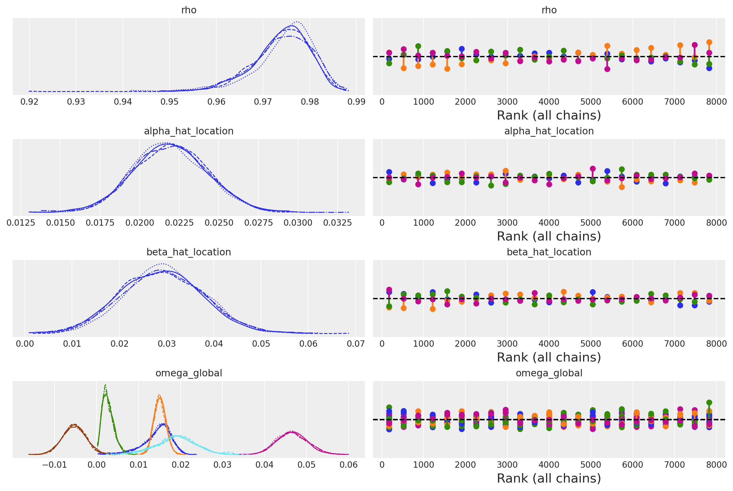
../_images/0973c34fb7f535c89c51d3f0de40d7b80c4c679fad12957b3cf064fb912b3160.png

Next we’ll look at some of the summary statistics and how they vary across the countries.

az.summary(
    idata_full_test,
    var_names=[
        "rho",
        "alpha_hat_location",
        "alpha_hat_scale",
        "beta_hat_location",
        "beta_hat_scale",
        "z_scale_alpha_Ireland",
        "z_scale_alpha_United States",
        "z_scale_beta_Ireland",
        "z_scale_beta_United States",
        "alpha_Ireland",
        "alpha_United States",
        "omega_global_corr",
        "lag_coefs_Ireland",
        "lag_coefs_United States",
    ],
)

/Users/nathanielforde/mambaforge/envs/myjlabenv/lib/python3.11/site-packages/arviz/stats/diagnostics.py:584: RuntimeWarning: invalid value encountered in scalar divide
  (between_chain_variance / within_chain_variance + num_samples - 1) / (num_samples)

	mean	sd	hdi_3%	hdi_97%	mcse_mean	mcse_sd	ess_bulk	ess_tail	r_hat
rho	0.974	0.006	0.962	0.984	0.000	0.000	749.0	1354.0	1.00
alpha_hat_location	0.022	0.002	0.018	0.026	0.000	0.000	1642.0	3651.0	1.00
alpha_hat_scale	0.047	0.012	0.027	0.069	0.000	0.000	2933.0	1097.0	1.00
beta_hat_location	0.029	0.009	0.014	0.046	0.000	0.000	855.0	2218.0	1.00
beta_hat_scale	0.186	0.064	0.077	0.305	0.003	0.002	312.0	647.0	1.01
z_scale_alpha_Ireland	0.264	0.147	0.070	0.508	0.002	0.002	2074.0	854.0	1.00
z_scale_alpha_United States	0.132	0.066	0.045	0.245	0.001	0.001	8457.0	5680.0	1.00
z_scale_beta_Ireland	0.508	0.326	0.096	1.067	0.014	0.010	592.0	1294.0	1.00
z_scale_beta_United States	0.213	0.125	0.050	0.445	0.005	0.003	646.0	1423.0	1.00
alpha_Ireland[dl_gdp]	0.035	0.008	0.020	0.048	0.000	0.000	3446.0	4001.0	1.00
alpha_Ireland[dl_cons]	0.014	0.006	0.003	0.024	0.000	0.000	1597.0	4464.0	1.00
alpha_Ireland[dl_gfcf]	0.024	0.011	0.002	0.046	0.000	0.000	6768.0	5217.0	1.00
alpha_United States[dl_gdp]	0.021	0.003	0.015	0.026	0.000	0.000	2322.0	3773.0	1.00
alpha_United States[dl_cons]	0.020	0.003	0.015	0.025	0.000	0.000	2164.0	3321.0	1.00
alpha_United States[dl_gfcf]	0.024	0.005	0.015	0.034	0.000	0.000	4455.0	5176.0	1.00
omega_global_corr[0, 0]	1.000	0.000	1.000	1.000	0.000	0.000	8000.0	8000.0	NaN
omega_global_corr[0, 1]	0.980	0.019	0.944	1.000	0.000	0.000	2393.0	2273.0	1.00
omega_global_corr[0, 2]	0.916	0.033	0.854	0.977	0.001	0.001	915.0	763.0	1.00
omega_global_corr[1, 0]	0.980	0.019	0.944	1.000	0.000	0.000	2393.0	2273.0	1.00
omega_global_corr[1, 1]	1.000	0.000	1.000	1.000	0.000	0.000	7937.0	7898.0	1.00
omega_global_corr[1, 2]	0.879	0.045	0.794	0.960	0.001	0.001	1345.0	3018.0	1.00
omega_global_corr[2, 0]	0.916	0.033	0.854	0.977	0.001	0.001	915.0	763.0	1.00
omega_global_corr[2, 1]	0.879	0.045	0.794	0.960	0.001	0.001	1345.0	3018.0	1.00
omega_global_corr[2, 2]	1.000	0.000	1.000	1.000	0.000	0.000	8042.0	7890.0	1.00
lag_coefs_Ireland[dl_gdp, 1, dl_gdp]	0.012	0.080	-0.151	0.160	0.001	0.001	5559.0	3646.0	1.00
lag_coefs_Ireland[dl_gdp, 1, dl_cons]	0.007	0.086	-0.161	0.174	0.001	0.002	4661.0	3294.0	1.00
lag_coefs_Ireland[dl_gdp, 1, dl_gfcf]	0.057	0.037	-0.009	0.128	0.001	0.000	4699.0	4249.0	1.00
lag_coefs_Ireland[dl_gdp, 2, dl_gdp]	-0.005	0.087	-0.176	0.152	0.002	0.002	3099.0	2447.0	1.00
lag_coefs_Ireland[dl_gdp, 2, dl_cons]	0.003	0.088	-0.171	0.171	0.001	0.001	4239.0	2997.0	1.00
lag_coefs_Ireland[dl_gdp, 2, dl_gfcf]	0.104	0.041	0.027	0.180	0.001	0.001	1785.0	4172.0	1.00
lag_coefs_Ireland[dl_cons, 1, dl_gdp]	0.132	0.081	-0.000	0.287	0.002	0.002	1109.0	1022.0	1.00
lag_coefs_Ireland[dl_cons, 1, dl_cons]	0.158	0.110	-0.004	0.376	0.003	0.002	1227.0	2390.0	1.00
lag_coefs_Ireland[dl_cons, 1, dl_gfcf]	-0.031	0.028	-0.082	0.023	0.001	0.000	1756.0	4031.0	1.00
lag_coefs_Ireland[dl_cons, 2, dl_gdp]	0.018	0.069	-0.120	0.147	0.001	0.001	5040.0	3039.0	1.00
lag_coefs_Ireland[dl_cons, 2, dl_cons]	0.048	0.073	-0.095	0.189	0.001	0.001	5765.0	3448.0	1.00
lag_coefs_Ireland[dl_cons, 2, dl_gfcf]	0.071	0.025	0.021	0.116	0.000	0.000	5169.0	5742.0	1.00
lag_coefs_Ireland[dl_gfcf, 1, dl_gdp]	0.091	0.118	-0.094	0.332	0.003	0.002	2232.0	1385.0	1.00
lag_coefs_Ireland[dl_gfcf, 1, dl_cons]	0.058	0.099	-0.136	0.254	0.002	0.002	5377.0	2440.0	1.00
lag_coefs_Ireland[dl_gfcf, 1, dl_gfcf]	0.064	0.076	-0.076	0.216	0.001	0.001	4693.0	3703.0	1.00
lag_coefs_Ireland[dl_gfcf, 2, dl_gdp]	0.050	0.092	-0.121	0.232	0.001	0.001	6475.0	3196.0	1.00
lag_coefs_Ireland[dl_gfcf, 2, dl_cons]	0.024	0.096	-0.154	0.221	0.001	0.002	5052.0	3012.0	1.00
lag_coefs_Ireland[dl_gfcf, 2, dl_gfcf]	-0.048	0.093	-0.239	0.102	0.002	0.002	1904.0	2237.0	1.00
lag_coefs_United States[dl_gdp, 1, dl_gdp]	0.033	0.044	-0.043	0.122	0.001	0.001	2364.0	1396.0	1.00
lag_coefs_United States[dl_gdp, 1, dl_cons]	0.031	0.042	-0.044	0.119	0.001	0.001	3946.0	2353.0	1.00
lag_coefs_United States[dl_gdp, 1, dl_gfcf]	-0.008	0.031	-0.072	0.043	0.001	0.001	1330.0	2254.0	1.00
lag_coefs_United States[dl_gdp, 2, dl_gdp]	0.036	0.042	-0.037	0.121	0.001	0.001	3903.0	2216.0	1.00
lag_coefs_United States[dl_gdp, 2, dl_cons]	0.048	0.047	-0.033	0.141	0.001	0.001	1335.0	1481.0	1.00
lag_coefs_United States[dl_gdp, 2, dl_gfcf]	0.027	0.028	-0.027	0.076	0.000	0.000	3760.0	1877.0	1.00
lag_coefs_United States[dl_cons, 1, dl_gdp]	0.024	0.041	-0.060	0.102	0.001	0.001	5468.0	2430.0	1.00
lag_coefs_United States[dl_cons, 1, dl_cons]	0.044	0.047	-0.031	0.141	0.001	0.001	1768.0	1738.0	1.00
lag_coefs_United States[dl_cons, 1, dl_gfcf]	0.007	0.031	-0.053	0.060	0.001	0.001	1909.0	2312.0	1.00
lag_coefs_United States[dl_cons, 2, dl_gdp]	0.039	0.044	-0.033	0.131	0.001	0.001	2644.0	1843.0	1.00
lag_coefs_United States[dl_cons, 2, dl_cons]	0.036	0.042	-0.040	0.116	0.001	0.001	4171.0	1978.0	1.00
lag_coefs_United States[dl_cons, 2, dl_gfcf]	0.031	0.027	-0.018	0.084	0.000	0.000	4192.0	2149.0	1.00
lag_coefs_United States[dl_gfcf, 1, dl_gdp]	0.039	0.045	-0.045	0.129	0.001	0.001	3809.0	1798.0	1.00
lag_coefs_United States[dl_gfcf, 1, dl_cons]	0.034	0.045	-0.046	0.125	0.001	0.001	4896.0	2476.0	1.00
lag_coefs_United States[dl_gfcf, 1, dl_gfcf]	0.075	0.057	-0.005	0.189	0.002	0.002	746.0	1317.0	1.00
lag_coefs_United States[dl_gfcf, 2, dl_gdp]	0.016	0.047	-0.078	0.102	0.001	0.001	4171.0	1975.0	1.00
lag_coefs_United States[dl_gfcf, 2, dl_cons]	0.018	0.047	-0.078	0.104	0.001	0.001	4508.0	1892.0	1.00
lag_coefs_United States[dl_gfcf, 2, dl_gfcf]	0.015	0.043	-0.072	0.091	0.001	0.001	2937.0	2034.0	1.00

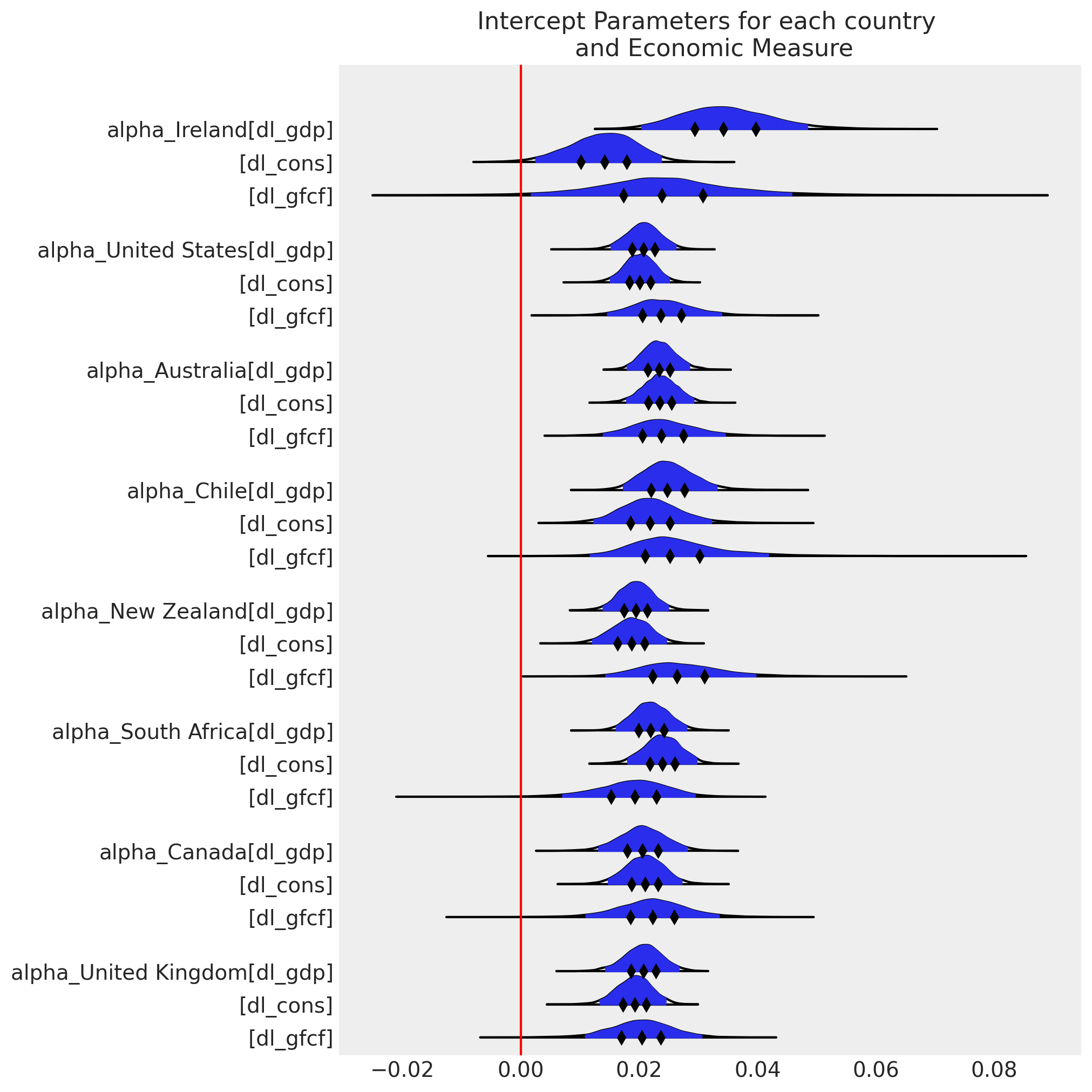
ax = az.plot_forest(
    idata_full_test,
    var_names=[
        "alpha_Ireland",
        "alpha_United States",
        "alpha_Australia",
        "alpha_Chile",
        "alpha_New Zealand",
        "alpha_South Africa",
        "alpha_Canada",
        "alpha_United Kingdom",
    ],
    kind="ridgeplot",
    combined=True,
    ridgeplot_truncate=False,
    ridgeplot_quantiles=[0.25, 0.5, 0.75],
    ridgeplot_overlap=0.7,
    figsize=(10, 10),
)

ax[0].axvline(0, color="red")
ax[0].set_title("Intercept Parameters for each country \n and Economic Measure");

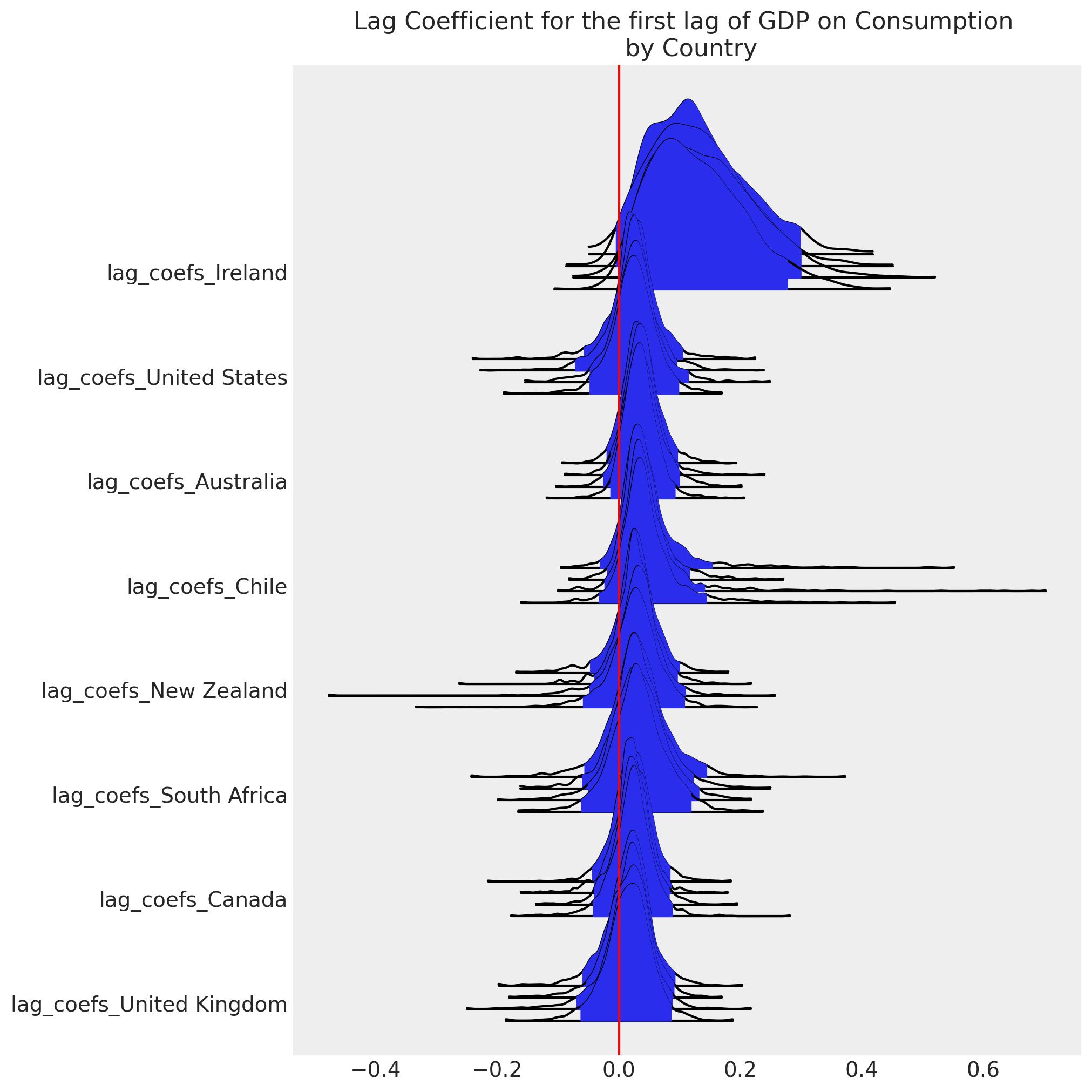
../_images/708fa57bc05b287a439ac2eca09319f05ef5d305b9ee154e8d123d4218038f75.png

ax = az.plot_forest(
    idata_full_test,
    var_names=[
        "lag_coefs_Ireland",
        "lag_coefs_United States",
        "lag_coefs_Australia",
        "lag_coefs_Chile",
        "lag_coefs_New Zealand",
        "lag_coefs_South Africa",
        "lag_coefs_Canada",
        "lag_coefs_United Kingdom",
    ],
    kind="ridgeplot",
    ridgeplot_truncate=False,
    figsize=(10, 10),
    coords={"equations": "dl_cons", "lags": 1, "cross_vars": "dl_gdp"},
)
ax[0].axvline(0, color="red")
ax[0].set_title("Lag Coefficient for the first lag of GDP on Consumption \n by Country");

../_images/f4266cc9962e37d1182e4cf1b48f5c995454b0223a7dd632eaa918b646cabf0a.png

Next we’ll examine the correlation between the three variables and see what we’ve learned by including the hierarchical structure.

corr = pd.DataFrame(
    az.summary(idata_full_test, var_names=["omega_global_corr"])["mean"].values.reshape(3, 3),
    columns=["GDP", "CONS", "GFCF"],
)
corr.index = ["GDP", "CONS", "GFCF"]
corr

/Users/nathanielforde/mambaforge/envs/myjlabenv/lib/python3.11/site-packages/arviz/stats/diagnostics.py:584: RuntimeWarning: invalid value encountered in scalar divide
  (between_chain_variance / within_chain_variance + num_samples - 1) / (num_samples)

	GDP	CONS	GFCF
GDP	1.000	0.980	0.916
CONS	0.980	1.000	0.879
GFCF	0.916	0.879	1.000

ax = az.plot_posterior(
    idata_full_test,
    var_names="omega_global_corr",
    hdi_prob="hide",
    point_estimate="mean",
    grid=(3, 3),
    kind="hist",
    ec="black",
    figsize=(10, 7),
)
titles = [
    "GDP/GDP",
    "GDP/CONS",
    "GDP/GFCF",
    "CONS/GDP",
    "CONS/CONS",
    "CONS/GFCF",
    "GFCF/GDP",
    "GFCF/CONS",
    "GFCF/GFCF",
]
for ax, t in zip(ax.ravel(), titles):
    ax.set_xlim(0.6, 1)
    ax.set_title(t, fontsize=10)
plt.suptitle("The Posterior Correlation Estimates", fontsize=20);

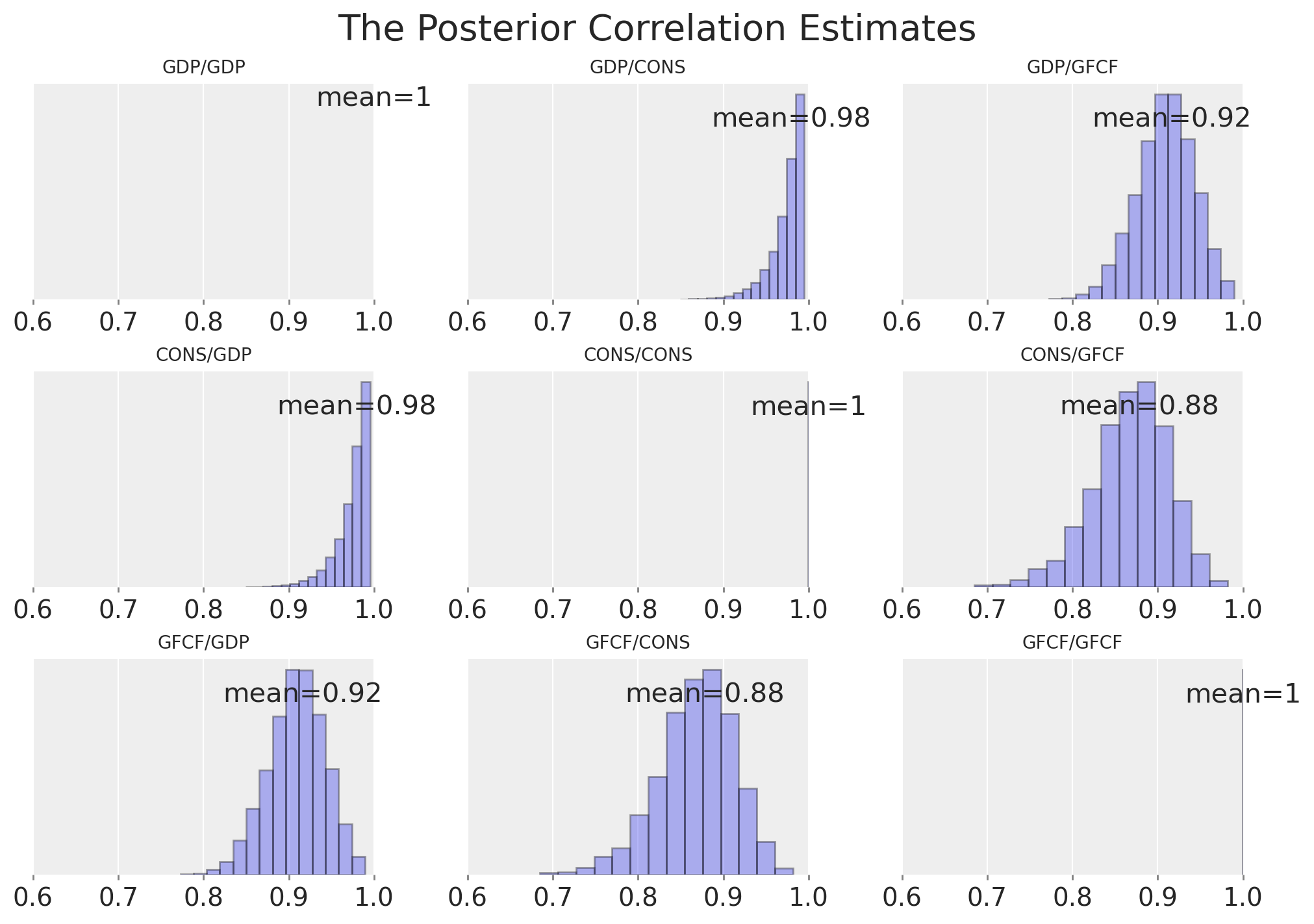
../_images/a9a547cae3a8bbee1dd7a1b0d7e2ee8c0291636e99c8a8cf17d4a6c6935367bf.png

We can see these estimates of the correlations between the 3 economic variables differ markedly from the simple case where we examined Ireland alone. In particular we can see that the correlation between GDF and CONS is now much higher. Which suggests that we have learned something about the relationship between these variables which would not be clear examining the Irish case alone.

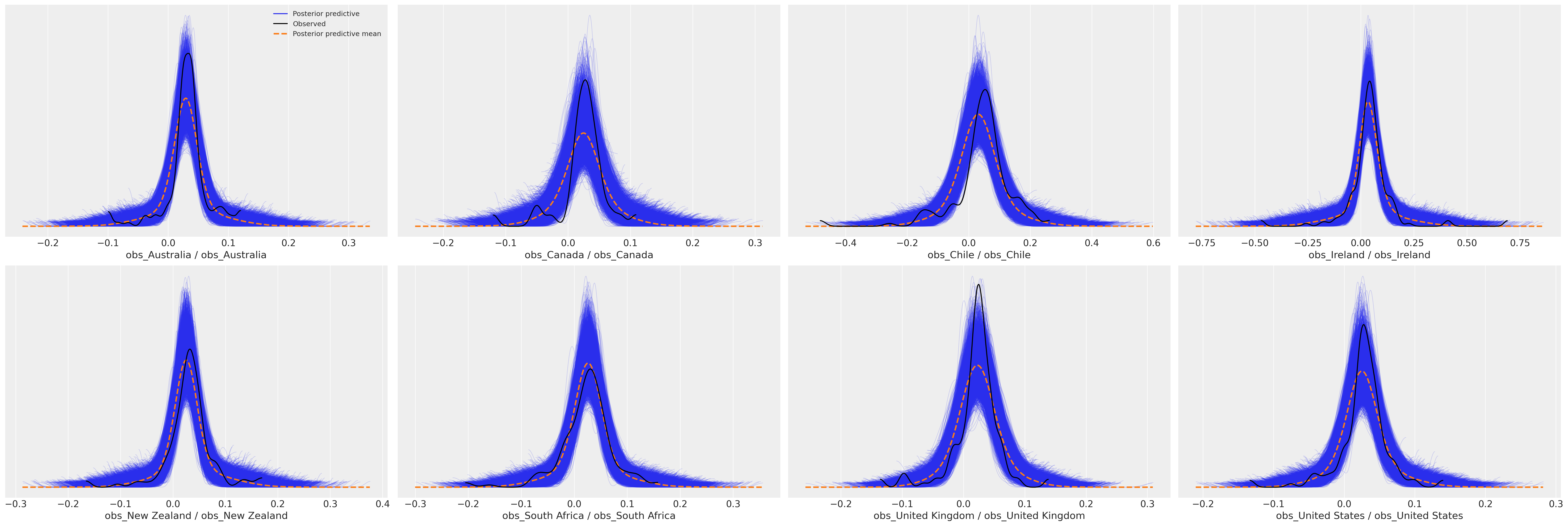
Next we’ll plot the model fits for each country to ensure that the predictive distribution can recover the observed data. It is important for the question of model adequacy that we can recover both the outlier case of Ireland and the more regular countries such as Australia and United States.

az.plot_ppc(idata_full_test);

../_images/7a35a2c85b92acdda41eba93f1ac78df2f1eb882a02229d33a76dbd30ff4153c.png

And to see the development of these model fits over time:

countries = gdp_hierarchical["country"].unique()


fig, axs = plt.subplots(8, 3, figsize=(20, 40))
for ax, country in zip(axs, countries):
    temp = pd.DataFrame(
        idata_full_test["observed_data"][f"obs_{country}"].data,
        columns=["dl_gdp", "dl_cons", "dl_gfcf"],
    )
    ppc = az.extract(idata_full_test, group="posterior_predictive", num_samples=100)[
        f"obs_{country}"
    ]
    if country == "Ireland":
        color = "viridis"
    else:
        color = "inferno"
    for i in range(3):
        shade_background(ppc, ax, i, color)
    ax[0].plot(np.arange(ppc.shape[0]), ppc[:, 0, :].mean(axis=1), color="cyan", label="Mean")
    ax[0].plot(temp["dl_gdp"], "o", mfc="black", mec="white", mew=1, markersize=7, label="Observed")
    ax[0].set_title(f"Posterior Predictive GDP: {country}")
    ax[0].legend(loc="lower left")
    ax[1].plot(
        temp["dl_cons"], "o", mfc="black", mec="white", mew=1, markersize=7, label="Observed"
    )
    ax[1].plot(np.arange(ppc.shape[0]), ppc[:, 1, :].mean(axis=1), color="cyan", label="Mean")
    ax[1].set_title(f"Posterior Predictive Consumption: {country}")
    ax[1].legend(loc="lower left")
    ax[2].plot(
        temp["dl_gfcf"], "o", mfc="black", mec="white", mew=1, markersize=7, label="Observed"
    )
    ax[2].plot(np.arange(ppc.shape[0]), ppc[:, 2, :].mean(axis=1), color="cyan", label="Mean")
    ax[2].set_title(f"Posterior Predictive Investment: {country}")
    ax[2].legend(loc="lower left")
plt.suptitle("Posterior Predictive Checks on Hierarchical VAR", fontsize=20);

../_images/24c70f66bf4247625c0651c404b9457dd1390ba05e1dd1d1e07485f64e71acd5.png

Here we can see that the model appears to have recovered reasonable posterior predictions for the observed data and the volatility of the Irish GDP figures is clear next to the other countries. Whether this is a cautionary tale about data quality or the corruption of metrics we leave to the economists to figure out.

Conclusion#

VAR modelling is a rich an interesting area of research within economics and there are a range of challenges and pitfalls which come with the interpretation and understanding of these models. We hope this example encourages you to continue exploring the potential of this kind of VAR modelling in the Bayesian framework. Whether you’re interested in the relationship between grand economic theory or simpler questions about the impact of poor app performance on customer feedback, VAR models give you a powerful tool for interrogating these relationships over time. As we’ve seen Hierarchical VARs further enables the precise quantification of outliers within a cohort and does not throw away the information because of odd accounting practices engendered by international capitalism.

In the next post in this series we will spend some time digging into the implied relationships between the timeseries which result from fitting our VAR models.

References#

[1]

Ricardo Vieira. Bayesian vector autoregression in pymc. URL: https://www.pymc-labs.io/blog-posts/bayesian-vector-autoregression/ (visited on 2022-12-09).

Authors#

Adapted from the PYMC labs Blog post and Jim Savage’s discussion here by Nathaniel Forde in November 2022 (pymc-examples#456)
Reexecuted by Nathaniel Forde on Feb, 2023 (pymc_examples#523)

Watermark#

%load_ext watermark
%watermark -n -u -v -iv -w -p pytensor,aeppl,xarray

Last updated: Tue Feb 21 2023

Python implementation: CPython
Python version       : 3.11.0
IPython version      : 8.9.0

pytensor: 2.8.11
aeppl   : not installed
xarray  : 2023.1.0

pymc       : 5.0.1
statsmodels: 0.13.5
pandas     : 1.5.3
numpy      : 1.24.1
matplotlib : 3.6.3
arviz      : 0.14.0

Watermark: 2.3.1

License notice#

All the notebooks in this example gallery are provided under the MIT License which allows modification, and redistribution for any use provided the copyright and license notices are preserved.

Citing PyMC examples#

To cite this notebook, use the DOI provided by Zenodo for the pymc-examples repository.

Important

Many notebooks are adapted from other sources: blogs, books… In such cases you should cite the original source as well.

Also remember to cite the relevant libraries used by your code.

Here is an citation template in bibtex:

@incollection{citekey,
  author    = "<notebook authors, see above>",
  title     = "<notebook title>",
  editor    = "PyMC Team",
  booktitle = "PyMC examples",
  doi       = "10.5281/zenodo.5654871"
}

which once rendered could look like:

Categories

Tags