Multivariate Gaussian Random Walk

import arviz as az
import matplotlib.pyplot as plt
import numpy as np
import pymc as pm
import pytensor

from scipy.linalg import cholesky

%matplotlib inline

RANDOM_SEED = 8927
rng = np.random.default_rng(RANDOM_SEED)
az.style.use("arviz-darkgrid")

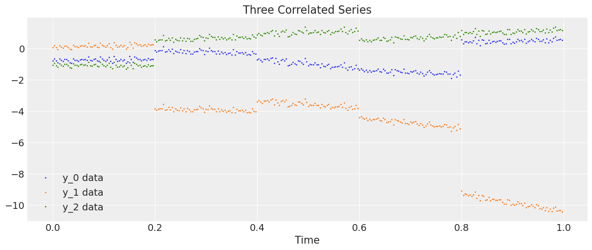
This notebook shows how to fit a correlated time series using multivariate Gaussian random walks (GRWs). In particular, we perform a Bayesian regression of the time series data against a model dependent on GRWs.

We generate data as the 3-dimensional time series

()\[ \mathbf y = \alpha_{i[\mathbf t]} +\beta_{i[\mathbf t]} *\frac{\mathbf t}{300} +\xi_{\mathbf t},\quad \mathbf t = [0,1,...,299], \]

where

• \(i\mapsto\alpha_{i}\) and \(i\mapsto\beta_{i}\), \(i\in\{0,1,2,3,4\}\), are two 3-dimensional Gaussian random walks for two correlation matrices \(\Sigma_\alpha\) and \(\Sigma_\beta\),

• we define the index $\( i[t]= j\quad\text{for}\quad t = 60j,60j+1,...,60j+59, \quad\text{and}\quad j = 0,1,2,3,4, \)$

• \(*\) means that we multiply the \(j\)-th column of the \(3\times300\) matrix with the \(j\)-th entry of the vector for each \(j=0,1,...,299\), and

• \(\xi_{\mathbf t}\) is a \(3\times300\) matrix with iid normal entries \(N(0,\sigma^2)\).

So the series \(\mathbf y\) changes due to the GRW \(\alpha\) in five occasions, namely steps \(0,60,120,180,240\). Meanwhile \(\mathbf y\) changes at steps \(1,60,120,180,240\) due to the increments of the GRW \(\beta\) and at every step due to the weighting of \(\beta\) with \(\mathbf t/300\). Intuitively, we have a noisy (\(\xi\)) system that is shocked five times over a period of 300 steps, but the impact of the \(\beta\) shocks gradually becomes more significant at every step.

Data generation

Let’s generate and plot the data.

D = 3  # Dimension of random walks
N = 300  # Number of steps
sections = 5  # Number of sections
period = N / sections  # Number steps in each section

Sigma_alpha = rng.standard_normal((D, D))
Sigma_alpha = Sigma_alpha.T.dot(Sigma_alpha)  # Construct covariance matrix for alpha
L_alpha = cholesky(Sigma_alpha, lower=True)  # Obtain its Cholesky decomposition

Sigma_beta = rng.standard_normal((D, D))
Sigma_beta = Sigma_beta.T.dot(Sigma_beta)  # Construct covariance matrix for beta
L_beta = cholesky(Sigma_beta, lower=True)  # Obtain its Cholesky decomposition

# Gaussian random walks:
alpha = np.cumsum(L_alpha.dot(rng.standard_normal((D, sections))), axis=1).T
beta = np.cumsum(L_beta.dot(rng.standard_normal((D, sections))), axis=1).T
t = np.arange(N)[:, None] / N
alpha = np.repeat(alpha, period, axis=0)
beta = np.repeat(beta, period, axis=0)
# Correlated series
sigma = 0.1
y = alpha + beta * t + sigma * rng.standard_normal((N, 1))

# Plot the correlated series
plt.figure(figsize=(12, 5))
plt.plot(t, y, ".", markersize=2, label=("y_0 data", "y_1 data", "y_2 data"))
plt.title("Three Correlated Series")
plt.xlabel("Time")
plt.legend()
plt.show();

Model

First we introduce a scaling class to rescale our data and the time parameter before the sampling and then rescale the predictions to match the unscaled data.

class Scaler:
    def __init__(self):
        mean_ = None
        std_ = None

    def transform(self, x):
        return (x - self.mean_) / self.std_

    def fit_transform(self, x):
        self.mean_ = x.mean(axis=0)
        self.std_ = x.std(axis=0)
        return self.transform(x)

    def inverse_transform(self, x):
        return x * self.std_ + self.mean_

We now construct the regression model in () imposing priors on the GRWs \(\alpha\) and \(\beta\), on the standard deviation \(\sigma\) and hyperpriors on the Cholesky matrices. We use the LKJ prior [Lewandowski et al., 2009] for the Cholesky matrices (see this link for the documentation and also the PyMC notebook /case_studies/LKJ for some usage examples.)

def inference(t, y, sections, n_samples=100):
    N, D = y.shape

    # Standardize y and t
    y_scaler = Scaler()
    t_scaler = Scaler()
    y = y_scaler.fit_transform(y)
    t = t_scaler.fit_transform(t)
    # Create a section index
    t_section = np.repeat(np.arange(sections), N / sections)

    # Create PyTensor equivalent
    t_t = pytensor.shared(np.repeat(t, D, axis=1))
    y_t = pytensor.shared(y)
    t_section_t = pytensor.shared(t_section)

    coords = {"y_": ["y_0", "y_1", "y_2"], "steps": np.arange(N)}
    with pm.Model(coords=coords) as model:
        # Hyperpriors on Cholesky matrices
        chol_alpha, *_ = pm.LKJCholeskyCov(
            "chol_cov_alpha", n=D, eta=2, sd_dist=pm.HalfCauchy.dist(2.5), compute_corr=True
        )
        chol_beta, *_ = pm.LKJCholeskyCov(
            "chol_cov_beta", n=D, eta=2, sd_dist=pm.HalfCauchy.dist(2.5), compute_corr=True
        )

        # Priors on Gaussian random walks
        alpha = pm.MvGaussianRandomWalk(
            "alpha", mu=np.zeros(D), chol=chol_alpha, shape=(sections, D)
        )
        beta = pm.MvGaussianRandomWalk("beta", mu=np.zeros(D), chol=chol_beta, shape=(sections, D))

        # Deterministic construction of the correlated random walk
        alpha_r = alpha[t_section_t]
        beta_r = beta[t_section_t]
        regression = alpha_r + beta_r * t_t

        # Prior on noise ξ
        sigma = pm.HalfNormal("sigma", 1.0)

        # Likelihood
        likelihood = pm.Normal("y", mu=regression, sigma=sigma, observed=y_t, dims=("steps", "y_"))

        # MCMC sampling
        trace = pm.sample(n_samples, tune=1000, chains=4, target_accept=0.9)

        # Posterior predictive sampling
        pm.sample_posterior_predictive(trace, extend_inferencedata=True)

    return trace, y_scaler, t_scaler, t_section

Inference

We now sample from our model and we return the trace, the scaling functions for space and time and the scaled time index.

trace, y_scaler, t_scaler, t_section = inference(t, y, sections)

/Users/cfonnesbeck/mambaforge/envs/pie/lib/python3.9/site-packages/pymc/distributions/timeseries.py:345: UserWarning: Initial distribution not specified, defaulting to `MvNormal.dist(0, I*100)`.You can specify an init_dist manually to suppress this warning.
  warnings.warn(
/Users/cfonnesbeck/mambaforge/envs/pie/lib/python3.9/site-packages/pymc/distributions/timeseries.py:345: UserWarning: Initial distribution not specified, defaulting to `MvNormal.dist(0, I*100)`.You can specify an init_dist manually to suppress this warning.
  warnings.warn(
Only 100 samples in chain.
/Users/cfonnesbeck/mambaforge/envs/pie/lib/python3.9/site-packages/pymc/logprob/joint_logprob.py:167: UserWarning: Found a random variable that was neither among the observations nor the conditioned variables: [multivariate_normal_rv{1, (1, 2), floatX, False}.0, multivariate_normal_rv{1, (1, 2), floatX, False}.out]
  warnings.warn(
/Users/cfonnesbeck/mambaforge/envs/pie/lib/python3.9/site-packages/pymc/logprob/joint_logprob.py:167: UserWarning: Found a random variable that was neither among the observations nor the conditioned variables: [multivariate_normal_rv{1, (1, 2), floatX, False}.0, multivariate_normal_rv{1, (1, 2), floatX, False}.out]
  warnings.warn(
/Users/cfonnesbeck/mambaforge/envs/pie/lib/python3.9/site-packages/pymc/logprob/joint_logprob.py:167: UserWarning: Found a random variable that was neither among the observations nor the conditioned variables: [multivariate_normal_rv{1, (1, 2), floatX, False}.0, multivariate_normal_rv{1, (1, 2), floatX, False}.out]
  warnings.warn(
/Users/cfonnesbeck/mambaforge/envs/pie/lib/python3.9/site-packages/pymc/logprob/joint_logprob.py:167: UserWarning: Found a random variable that was neither among the observations nor the conditioned variables: [multivariate_normal_rv{1, (1, 2), floatX, False}.0, multivariate_normal_rv{1, (1, 2), floatX, False}.out]
  warnings.warn(
/Users/cfonnesbeck/mambaforge/envs/pie/lib/python3.9/site-packages/multipledispatch/dispatcher.py:27: AmbiguityWarning: 
Ambiguities exist in dispatched function _unify

The following signatures may result in ambiguous behavior:
	[ConstrainedVar, Var, Mapping], [object, ConstrainedVar, Mapping]
	[object, ConstrainedVar, Mapping], [ConstrainedVar, object, Mapping]
	[object, ConstrainedVar, Mapping], [ConstrainedVar, Var, Mapping]
	[ConstrainedVar, object, Mapping], [object, ConstrainedVar, Mapping]


Consider making the following additions:

@dispatch(ConstrainedVar, ConstrainedVar, Mapping)
def _unify(...)

@dispatch(ConstrainedVar, ConstrainedVar, Mapping)
def _unify(...)

@dispatch(ConstrainedVar, ConstrainedVar, Mapping)
def _unify(...)

@dispatch(ConstrainedVar, ConstrainedVar, Mapping)
def _unify(...)
  warn(warning_text(dispatcher.name, ambiguities), AmbiguityWarning)
Auto-assigning NUTS sampler...
Initializing NUTS using jitter+adapt_diag...
/Users/cfonnesbeck/mambaforge/envs/pie/lib/python3.9/site-packages/pymc/logprob/joint_logprob.py:167: UserWarning: Found a random variable that was neither among the observations nor the conditioned variables: [multivariate_normal_rv{1, (1, 2), floatX, False}.0, multivariate_normal_rv{1, (1, 2), floatX, False}.out]
  warnings.warn(
/Users/cfonnesbeck/mambaforge/envs/pie/lib/python3.9/site-packages/pymc/logprob/joint_logprob.py:167: UserWarning: Found a random variable that was neither among the observations nor the conditioned variables: [multivariate_normal_rv{1, (1, 2), floatX, False}.0, multivariate_normal_rv{1, (1, 2), floatX, False}.out]
  warnings.warn(
/Users/cfonnesbeck/mambaforge/envs/pie/lib/python3.9/site-packages/pymc/logprob/joint_logprob.py:167: UserWarning: Found a random variable that was neither among the observations nor the conditioned variables: [multivariate_normal_rv{1, (1, 2), floatX, False}.0, multivariate_normal_rv{1, (1, 2), floatX, False}.out]
  warnings.warn(
/Users/cfonnesbeck/mambaforge/envs/pie/lib/python3.9/site-packages/pymc/logprob/joint_logprob.py:167: UserWarning: Found a random variable that was neither among the observations nor the conditioned variables: [multivariate_normal_rv{1, (1, 2), floatX, False}.0, multivariate_normal_rv{1, (1, 2), floatX, False}.out]
  warnings.warn(
/Users/cfonnesbeck/mambaforge/envs/pie/lib/python3.9/site-packages/pymc/logprob/joint_logprob.py:167: UserWarning: Found a random variable that was neither among the observations nor the conditioned variables: [multivariate_normal_rv{1, (1, 2), floatX, False}.0, multivariate_normal_rv{1, (1, 2), floatX, False}.out]
  warnings.warn(
/Users/cfonnesbeck/mambaforge/envs/pie/lib/python3.9/site-packages/pymc/logprob/joint_logprob.py:167: UserWarning: Found a random variable that was neither among the observations nor the conditioned variables: [multivariate_normal_rv{1, (1, 2), floatX, False}.0, multivariate_normal_rv{1, (1, 2), floatX, False}.out]
  warnings.warn(
/Users/cfonnesbeck/mambaforge/envs/pie/lib/python3.9/site-packages/pymc/logprob/joint_logprob.py:167: UserWarning: Found a random variable that was neither among the observations nor the conditioned variables: [multivariate_normal_rv{1, (1, 2), floatX, False}.0, multivariate_normal_rv{1, (1, 2), floatX, False}.out]
  warnings.warn(
/Users/cfonnesbeck/mambaforge/envs/pie/lib/python3.9/site-packages/pymc/logprob/joint_logprob.py:167: UserWarning: Found a random variable that was neither among the observations nor the conditioned variables: [multivariate_normal_rv{1, (1, 2), floatX, False}.0, multivariate_normal_rv{1, (1, 2), floatX, False}.out]
  warnings.warn(
/Users/cfonnesbeck/mambaforge/envs/pie/lib/python3.9/site-packages/pymc/logprob/joint_logprob.py:167: UserWarning: Found a random variable that was neither among the observations nor the conditioned variables: [multivariate_normal_rv{1, (1, 2), floatX, False}.0, multivariate_normal_rv{1, (1, 2), floatX, False}.out]
  warnings.warn(
/Users/cfonnesbeck/mambaforge/envs/pie/lib/python3.9/site-packages/pymc/logprob/joint_logprob.py:167: UserWarning: Found a random variable that was neither among the observations nor the conditioned variables: [multivariate_normal_rv{1, (1, 2), floatX, False}.0, multivariate_normal_rv{1, (1, 2), floatX, False}.out]
  warnings.warn(
/Users/cfonnesbeck/mambaforge/envs/pie/lib/python3.9/site-packages/pymc/logprob/joint_logprob.py:167: UserWarning: Found a random variable that was neither among the observations nor the conditioned variables: [multivariate_normal_rv{1, (1, 2), floatX, False}.0, multivariate_normal_rv{1, (1, 2), floatX, False}.out]
  warnings.warn(
/Users/cfonnesbeck/mambaforge/envs/pie/lib/python3.9/site-packages/pymc/logprob/joint_logprob.py:167: UserWarning: Found a random variable that was neither among the observations nor the conditioned variables: [multivariate_normal_rv{1, (1, 2), floatX, False}.0, multivariate_normal_rv{1, (1, 2), floatX, False}.out]
  warnings.warn(
/Users/cfonnesbeck/mambaforge/envs/pie/lib/python3.9/site-packages/pymc/logprob/joint_logprob.py:167: UserWarning: Found a random variable that was neither among the observations nor the conditioned variables: [multivariate_normal_rv{1, (1, 2), floatX, False}.0, multivariate_normal_rv{1, (1, 2), floatX, False}.out]
  warnings.warn(
/Users/cfonnesbeck/mambaforge/envs/pie/lib/python3.9/site-packages/pymc/logprob/joint_logprob.py:167: UserWarning: Found a random variable that was neither among the observations nor the conditioned variables: [multivariate_normal_rv{1, (1, 2), floatX, False}.0, multivariate_normal_rv{1, (1, 2), floatX, False}.out]
  warnings.warn(
/Users/cfonnesbeck/mambaforge/envs/pie/lib/python3.9/site-packages/pymc/logprob/joint_logprob.py:167: UserWarning: Found a random variable that was neither among the observations nor the conditioned variables: [multivariate_normal_rv{1, (1, 2), floatX, False}.0, multivariate_normal_rv{1, (1, 2), floatX, False}.out]
  warnings.warn(
/Users/cfonnesbeck/mambaforge/envs/pie/lib/python3.9/site-packages/pymc/logprob/joint_logprob.py:167: UserWarning: Found a random variable that was neither among the observations nor the conditioned variables: [multivariate_normal_rv{1, (1, 2), floatX, False}.0, multivariate_normal_rv{1, (1, 2), floatX, False}.out]
  warnings.warn(
/Users/cfonnesbeck/mambaforge/envs/pie/lib/python3.9/site-packages/pymc/logprob/joint_logprob.py:167: UserWarning: Found a random variable that was neither among the observations nor the conditioned variables: [multivariate_normal_rv{1, (1, 2), floatX, False}.0, multivariate_normal_rv{1, (1, 2), floatX, False}.out]
  warnings.warn(
/Users/cfonnesbeck/mambaforge/envs/pie/lib/python3.9/site-packages/pymc/logprob/joint_logprob.py:167: UserWarning: Found a random variable that was neither among the observations nor the conditioned variables: [multivariate_normal_rv{1, (1, 2), floatX, False}.0, multivariate_normal_rv{1, (1, 2), floatX, False}.out]
  warnings.warn(
Multiprocess sampling (4 chains in 4 jobs)
NUTS: [chol_cov_alpha, chol_cov_beta, alpha, beta, sigma]

100.00% [4400/4400 01:56<00:00 Sampling 4 chains, 0 divergences]

Sampling 4 chains for 1_000 tune and 100 draw iterations (4_000 + 400 draws total) took 118 seconds.
Sampling: [y]

100.00% [400/400 00:00<00:00]

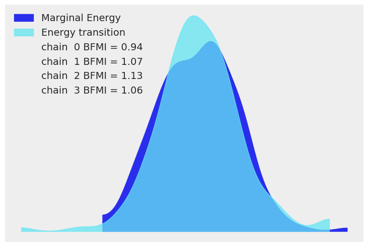
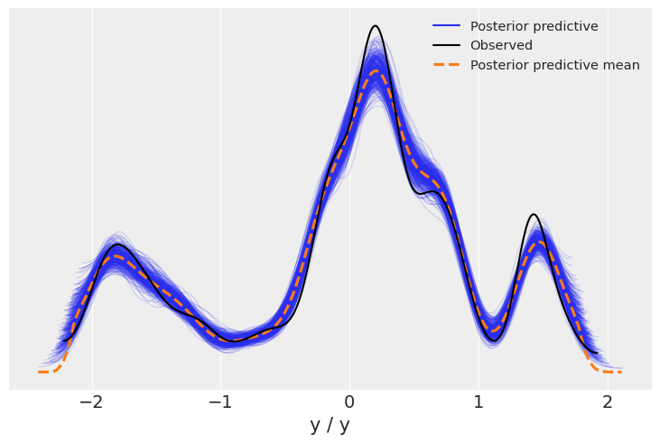
We now display the energy plot using arviz.plot_energy() for a visual check for the model’s convergence. Then, using arviz.plot_ppc(), we plot the distribution of the posterior predictive samples against the observed data \(\mathbf y\). This plot provides a general idea of the accuracy of the model (note that the values of \(\mathbf y\) actually correspond to the scaled version of \(\mathbf y\)).

az.plot_energy(trace)
az.plot_ppc(trace);

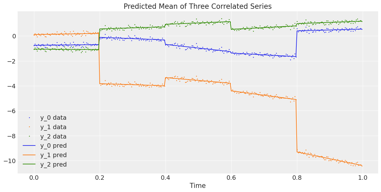
Posterior visualisation

The graphs above look good. Now we plot the observed 3-dimensional series against the average predicted 3-dimensional series, or in other words, we plot the data against the estimated regression curve from the model ().

# Compute the predicted mean of the multivariate GRWs
alpha_mean = trace.posterior["alpha"].mean(dim=("chain", "draw"))
beta_mean = trace.posterior["beta"].mean(dim=("chain", "draw"))

# Compute the predicted mean of the correlated series
y_pred = y_scaler.inverse_transform(
    alpha_mean[t_section].values + beta_mean[t_section].values * t_scaler.transform(t)
)

# Plot the predicted mean
fig, ax = plt.subplots(1, 1, figsize=(12, 6))
ax.plot(t, y, ".", markersize=2, label=("y_0 data", "y_1 data", "y_2 data"))
plt.gca().set_prop_cycle(None)
ax.plot(t, y_pred, label=("y_0 pred", "y_1 pred", "y_2 pred"))
ax.set_xlabel("Time")
ax.legend()
ax.set_title("Predicted Mean of Three Correlated Series");

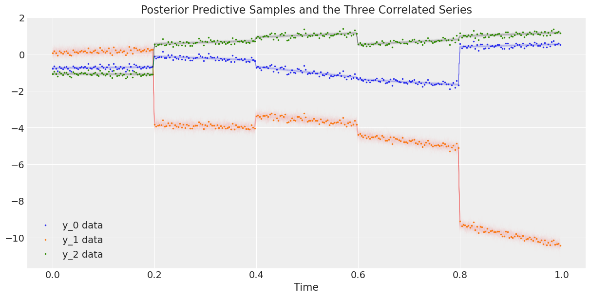
Finally, we plot the data against the posterior predictive samples.

# Rescale the posterior predictive samples
ppc_y = y_scaler.inverse_transform(trace.posterior_predictive["y"].mean("chain"))

fig, ax = plt.subplots(1, 1, figsize=(12, 6))
# Plot the data
ax.plot(t, y, ".", markersize=3, label=("y_0 data", "y_1 data", "y_2 data"))
# Plot the posterior predictive samples
ax.plot(t, ppc_y.sel(y_="y_0").T, color="C0", alpha=0.003)
ax.plot(t, ppc_y.sel(y_="y_1").T, color="C1", alpha=0.003)
ax.plot(t, ppc_y.sel(y_="y_2").T, color="C2", alpha=0.003)
ax.set_xlabel("Time")
ax.legend()
ax.set_title("Posterior Predictive Samples and the Three Correlated Series");

Authors

• updated to best practices by Lorenzon Itoniazzi in October, 2021 (pymc-examples#195)

• updated to v5 by Chris Fonnesbeck in February, 2023

References

[1]

Daniel Lewandowski, Dorota Kurowicka, and Harry Joe. Generating random correlation matrices based on vines and extended onion method. Journal of multivariate analysis, 100(9):1989–2001, 2009.

Watermark

%load_ext watermark
%watermark -n -u -v -iv -w -p theano,xarray

Last updated: Thu Feb 02 2023

Python implementation: CPython
Python version       : 3.9.15
IPython version      : 8.7.0

theano: not installed
xarray: 2022.12.0

pytensor  : 2.8.11
numpy     : 1.23.5
pymc      : 5.0.1
sys       : 3.9.15 | packaged by conda-forge | (main, Nov 22 2022, 08:48:25) 
[Clang 14.0.6 ]
matplotlib: 3.6.2
arviz     : 0.14.0

Watermark: 2.3.1

License notice

All the notebooks in this example gallery are provided under the MIT License which allows modification, and redistribution for any use provided the copyright and license notices are preserved.

Citing PyMC examples

To cite this notebook, use the DOI provided by Zenodo for the pymc-examples repository.

Important

Many notebooks are adapted from other sources: blogs, books… In such cases you should cite the original source as well.

Also remember to cite the relevant libraries used by your code.

Here is an citation template in bibtex:

@incollection{citekey,
  author    = "<notebook authors, see above>",
  title     = "<notebook title>",
  editor    = "PyMC Team",
  booktitle = "PyMC examples",
  doi       = "10.5281/zenodo.5654871"
}

which once rendered could look like: