


Analysis of An \(AR(1)\) Model in PyMC#
import arviz as az
import matplotlib.pyplot as plt
import numpy as np
import pymc as pm
%config InlineBackend.figure_format = 'retina'
RANDOM_SEED = 8927
np.random.seed(RANDOM_SEED)
az.style.use("arviz-darkgrid")
Consider the following AR(2) process, initialized in the infinite past:
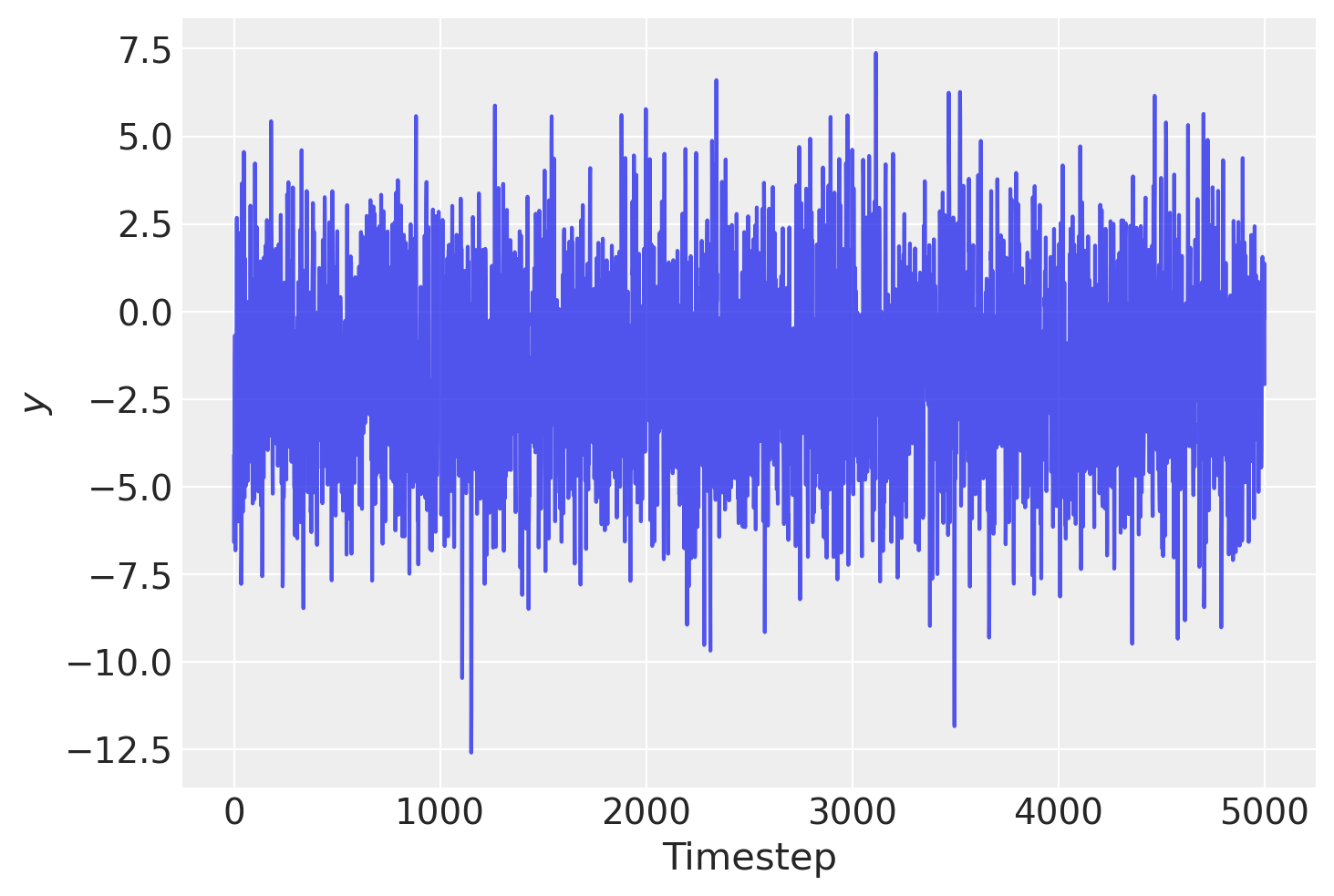
First, let’s generate some synthetic sample data. We simulate the ‘infinite past’ by generating 10,000 samples from an AR(2) process and then discarding the first 5,000:
T = 10000

# true stationarity:
true_rho = 0.7, -0.3
# true standard deviation of the innovation:
true_sigma = 2.0
# true process mean:
true_center = -1.0

y = np.random.normal(loc=true_center, scale=true_sigma, size=T)
y[1] += true_rho[0] * y[0]
for t in range(2, T - 100):
    y[t] += true_rho[0] * y[t - 1] + true_rho[1] * y[t - 2]

y = y[-5000:]
plt.plot(y, alpha=0.8)
plt.xlabel("Timestep")
plt.ylabel("$y$");
Let’s start by trying to fit the wrong model! Assume that we do no know the generative model and so simply fit an AR(1) model for simplicity.
This generative process is quite straight forward to implement in PyMC. Since we wish to include an intercept term in the AR process, we must set constant=True otherwise PyMC will assume that we want an AR2 process when rho is of size 2. Also, by default a \(N(0, 100)\) distribution will be used as the prior for the initial value. We can override this by passing a distribution (not a full RV) to the init_dist argument.
with pm.Model() as ar1:
    # assumes 95% of prob mass is between -2 and 2
    rho = pm.Normal("rho", mu=0.0, sigma=1.0, shape=2)
    # precision of the innovation term
    tau = pm.Exponential("tau", lam=0.5)

    likelihood = pm.AR(
        "y", rho=rho, tau=tau, constant=True, init_dist=pm.Normal.dist(0, 10), observed=y
    )

    idata = pm.sample(1000, tune=2000, random_seed=RANDOM_SEED)
Auto-assigning NUTS sampler...
Initializing NUTS using jitter+adapt_diag...
Multiprocess sampling (4 chains in 4 jobs)
NUTS: [rho, tau]
Sampling 4 chains for 2_000 tune and 1_000 draw iterations (8_000 + 4_000 draws total) took 5 seconds.
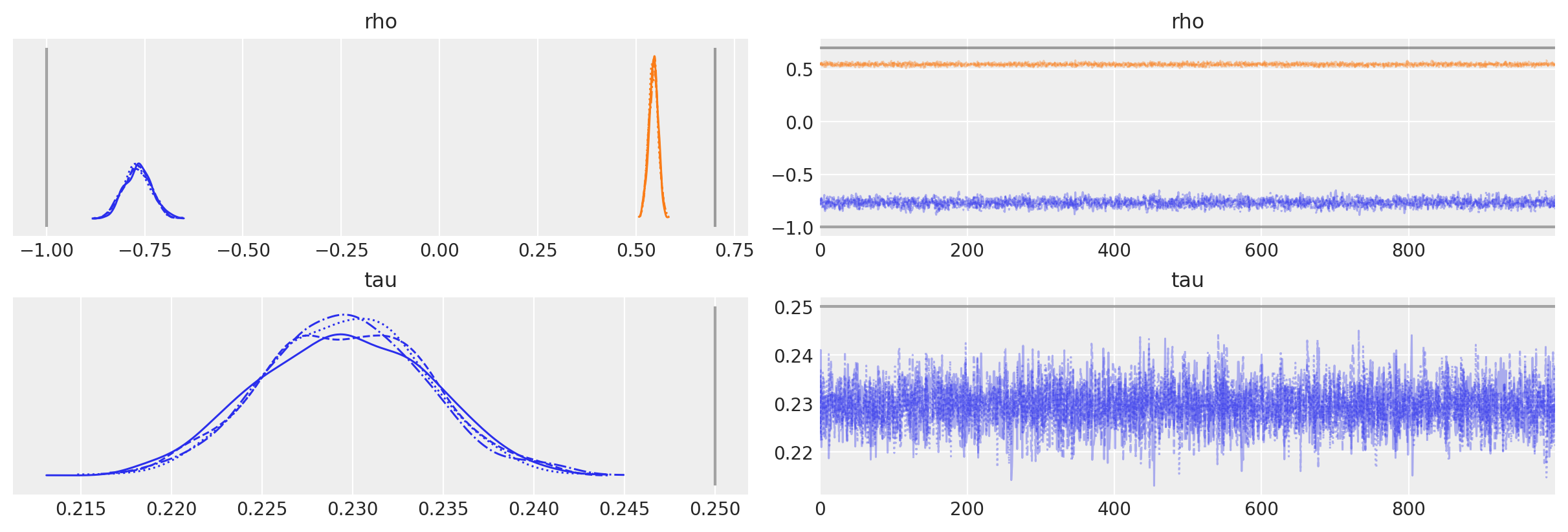
We can see that even though we assumed the wrong model, the parameter estimates are actually not that far from the true values.
az.plot_trace(
    idata,
    lines=[
        ("rho", {}, [true_center, true_rho[0]]),
        ("tau", {}, true_sigma**-2),
    ],
);
Extension to AR(p)#
Now let’s fit the correct underlying model, an AR(2):
The AR distribution infers the order of the process thanks to the size the of rho argument passed to AR (including the mean).
We will also use the standard deviation of the innovations (rather than the precision) to parameterize the distribution.
with pm.Model() as ar2:
    rho = pm.Normal("rho", 0.0, 1.0, shape=3)
    sigma = pm.HalfNormal("sigma", 3)
    likelihood = pm.AR(
        "y", rho=rho, sigma=sigma, constant=True, init_dist=pm.Normal.dist(0, 10), observed=y
    )

    idata = pm.sample(
        1000,
        tune=2000,
        random_seed=RANDOM_SEED,
    )
Auto-assigning NUTS sampler...
Initializing NUTS using jitter+adapt_diag...
Multiprocess sampling (4 chains in 4 jobs)
NUTS: [rho, sigma]
Sampling 4 chains for 2_000 tune and 1_000 draw iterations (8_000 + 4_000 draws total) took 9 seconds.
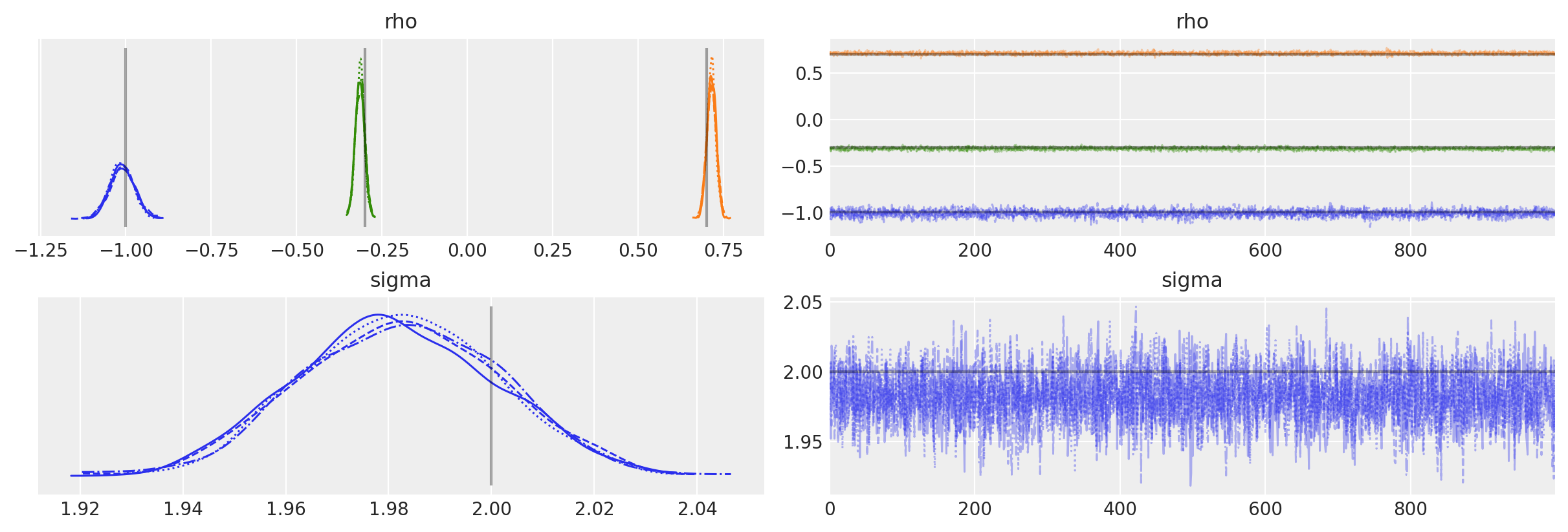
The posterior plots show that we have correctly inferred the generative model parameters.
az.plot_trace(
    idata,
    lines=[
        ("rho", {}, (true_center,) + true_rho),
        ("sigma", {}, true_sigma),
    ],
);
You can also pass the set of AR parameters as a list, if they are not identically distributed.
import pytensor.tensor as pt

with pm.Model() as ar2_bis:
    rho0 = pm.Normal("rho0", mu=0.0, sigma=5.0)
    rho1 = pm.Uniform("rho1", -1, 1)
    rho2 = pm.Uniform("rho2", -1, 1)
    sigma = pm.HalfNormal("sigma", 3)
    likelihood = pm.AR(
        "y",
        rho=pt.stack([rho0, rho1, rho2]),
        sigma=sigma,
        constant=True,
        init_dist=pm.Normal.dist(0, 10),
        observed=y,
    )

    idata = pm.sample(
        1000,
        tune=2000,
        target_accept=0.9,
        random_seed=RANDOM_SEED,
    )
Auto-assigning NUTS sampler...
Initializing NUTS using jitter+adapt_diag...
Multiprocess sampling (4 chains in 4 jobs)
NUTS: [rho0, rho1, rho2, sigma]
Sampling 4 chains for 2_000 tune and 1_000 draw iterations (8_000 + 4_000 draws total) took 10 seconds.
az.plot_trace(
    idata,
    lines=[
        ("rho0", {}, true_center),
        ("rho1", {}, true_rho[0]),
        ("rho2", {}, true_rho[1]),
        ("sigma", {}, true_sigma),
    ],
);

License notice#
All the notebooks in this example gallery are provided under the MIT License which allows modification, and redistribution for any use provided the copyright and license notices are preserved.
Citing PyMC examples#
To cite this notebook, use the DOI provided by Zenodo for the pymc-examples repository.
Important
Many notebooks are adapted from other sources: blogs, books… In such cases you should cite the original source as well.
Also remember to cite the relevant libraries used by your code.
Here is an citation template in bibtex:
@incollection{citekey,
  author    = "<notebook authors, see above>",
  title     = "<notebook title>",
  editor    = "PyMC Team",
  booktitle = "PyMC examples",
  doi       = "10.5281/zenodo.5654871"
}
which once rendered could look like: