Censored Data Models

from copy import copy

import arviz as az
import matplotlib.pyplot as plt
import numpy as np
import pymc as pm
import seaborn as sns

from numpy.random import default_rng

%config InlineBackend.figure_format = 'retina'
rng = default_rng(1234)
az.style.use("arviz-darkgrid")

This example notebook on Bayesian survival analysis touches on the point of censored data. Censoring is a form of missing-data problem, in which observations greater than a certain threshold are clipped down to that threshold, or observations less than a certain threshold are clipped up to that threshold, or both. These are called right, left and interval censoring, respectively. In this example notebook we consider interval censoring.

Censored data arises in many modelling problems. Two common examples are:

1. Survival analysis: when studying the effect of a certain medical treatment on survival times, it is impossible to prolong the study until all subjects have died. At the end of the study, the only data collected for many patients is that they were still alive for a time period \(T\) after the treatment was administered: in reality, their true survival times are greater than \(T\).

2. Sensor saturation: a sensor might have a limited range and the upper and lower limits would simply be the highest and lowest values a sensor can report. For instance, many mercury thermometers only report a very narrow range of temperatures.

This example notebook presents two different ways of dealing with censored data in PyMC3:

1. An imputed censored model, which represents censored data as parameters and makes up plausible values for all censored values. As a result of this imputation, this model is capable of generating plausible sets of made-up values that would have been censored. Each censored element introduces a random variable.

2. An unimputed censored model, where the censored data are integrated out and accounted for only through the log-likelihood. This method deals more adequately with large amounts of censored data and converges more quickly.

To establish a baseline we compare to an uncensored model of the uncensored data.

# Produce normally distributed samples
size = 500
true_mu = 13.0
true_sigma = 5.0
samples = rng.normal(true_mu, true_sigma, size)

# Set censoring limits
low = 3.0
high = 16.0


def censor(x, low, high):
    x = copy(x)
    x[x <= low] = low
    x[x >= high] = high
    return x


# Censor samples
censored = censor(samples, low, high)

# Visualize uncensored and censored data
_, ax = plt.subplots(figsize=(10, 3))
edges = np.linspace(-5, 35, 30)
ax.hist(samples, bins=edges, density=True, histtype="stepfilled", alpha=0.2, label="Uncensored")
ax.hist(censored, bins=edges, density=True, histtype="stepfilled", alpha=0.2, label="Censored")
[ax.axvline(x=x, c="k", ls="--") for x in [low, high]]
ax.legend();

Uncensored Model

def uncensored_model(data):
    with pm.Model() as model:
        mu = pm.Normal("mu", mu=((high - low) / 2) + low, sigma=(high - low))
        sigma = pm.HalfNormal("sigma", sigma=(high - low) / 2.0)
        observed = pm.Normal("observed", mu=mu, sigma=sigma, observed=data)
    return model

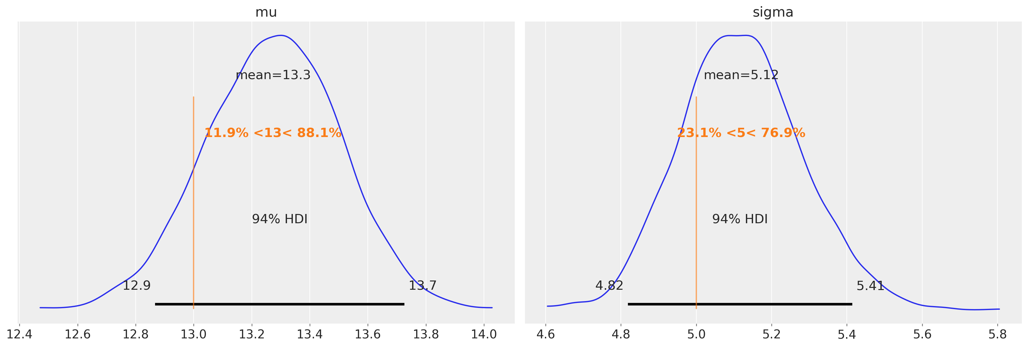
We should predict that running the uncensored model on uncensored data, we will get reasonable estimates of the mean and variance.

uncensored_model_1 = uncensored_model(samples)
with uncensored_model_1:
    idata = pm.sample()

az.plot_posterior(idata, ref_val=[true_mu, true_sigma], round_to=3);

Auto-assigning NUTS sampler...
Initializing NUTS using jitter+adapt_diag...
Multiprocess sampling (4 chains in 4 jobs)
NUTS: [mu, sigma]

100.00% [8000/8000 00:03<00:00 Sampling 4 chains, 0 divergences]

Sampling 4 chains for 1_000 tune and 1_000 draw iterations (4_000 + 4_000 draws total) took 4 seconds.

And that is exactly what we find.

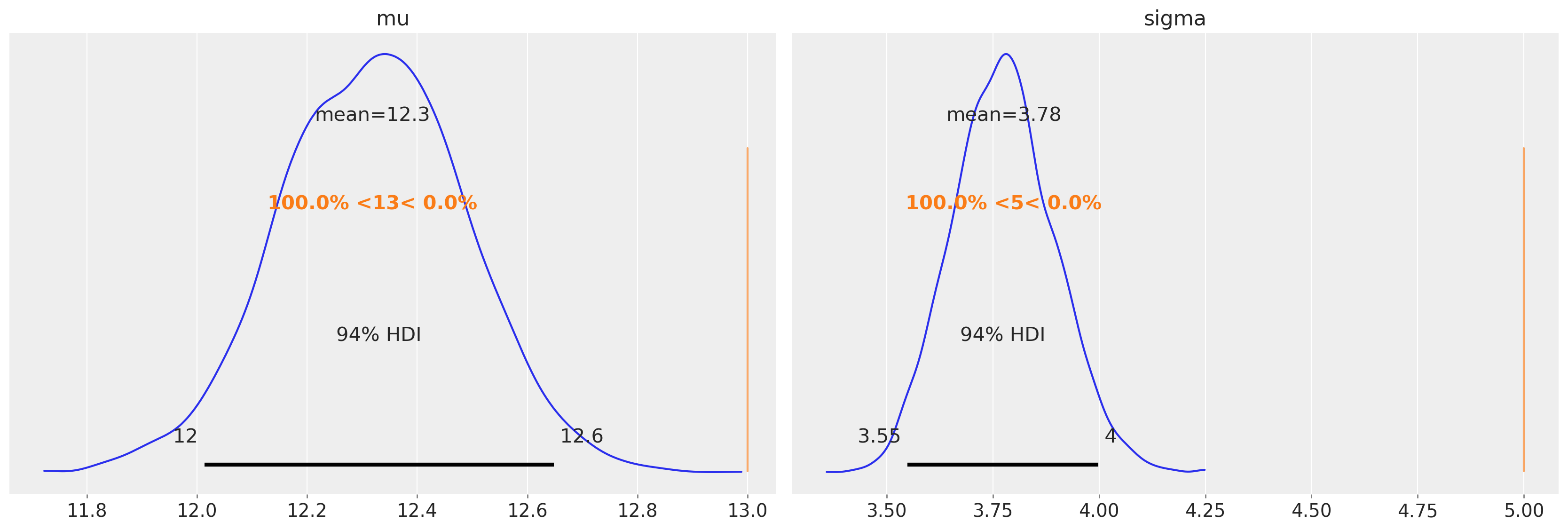
The problem however, is that in censored data contexts, we do not have access to the true values. If we were to use the same uncensored model on the censored data, we would anticipate that our parameter estimates will be biased. If we calculate point estimates for the mean and std, then we can see that we are likely to underestimate the mean and std for this particular dataset and censor bounds.

print(f"mean={np.mean(censored):.2f}; std={np.std(censored):.2f}")

mean=12.32; std=3.76

uncensored_model_2 = uncensored_model(censored)
with uncensored_model_2:
    idata = pm.sample()

az.plot_posterior(idata, ref_val=[true_mu, true_sigma], round_to=3);

Auto-assigning NUTS sampler...
Initializing NUTS using jitter+adapt_diag...
Multiprocess sampling (4 chains in 4 jobs)
NUTS: [mu, sigma]

100.00% [8000/8000 00:03<00:00 Sampling 4 chains, 0 divergences]

Sampling 4 chains for 1_000 tune and 1_000 draw iterations (4_000 + 4_000 draws total) took 4 seconds.

The figure above confirms this.

Censored data models

The models below show 2 approaches to dealing with censored data. First, we need to do a bit of data pre-processing to count the number of observations that are left or right censored. We also also need to extract just the non-censored data that we observe.

Model 1 - Imputed Censored Model of Censored Data

In this model, we impute the censored values from the same distribution as the uncensored data. Sampling from the posterior generates possible uncensored data sets.

n_right_censored = sum(censored >= high)
n_left_censored = sum(censored <= low)
n_observed = len(censored) - n_right_censored - n_left_censored
uncensored = censored[(censored > low) & (censored < high)]
assert len(uncensored) == n_observed

with pm.Model() as imputed_censored_model:
    mu = pm.Normal("mu", mu=((high - low) / 2) + low, sigma=(high - low))
    sigma = pm.HalfNormal("sigma", sigma=(high - low) / 2.0)
    right_censored = pm.Normal(
        "right_censored",
        mu,
        sigma,
        transform=pm.distributions.transforms.Interval(high, None),
        shape=int(n_right_censored),
        initval=np.full(n_right_censored, high + 1),
    )
    left_censored = pm.Normal(
        "left_censored",
        mu,
        sigma,
        transform=pm.distributions.transforms.Interval(None, low),
        shape=int(n_left_censored),
        initval=np.full(n_left_censored, low - 1),
    )
    observed = pm.Normal("observed", mu=mu, sigma=sigma, observed=uncensored, shape=int(n_observed))
    idata = pm.sample()

az.plot_posterior(idata, var_names=["mu", "sigma"], ref_val=[true_mu, true_sigma], round_to=3);

Auto-assigning NUTS sampler...
Initializing NUTS using jitter+adapt_diag...
Multiprocess sampling (4 chains in 4 jobs)
NUTS: [mu, sigma, right_censored, left_censored]

100.00% [8000/8000 00:16<00:00 Sampling 4 chains, 0 divergences]

Sampling 4 chains for 1_000 tune and 1_000 draw iterations (4_000 + 4_000 draws total) took 17 seconds.

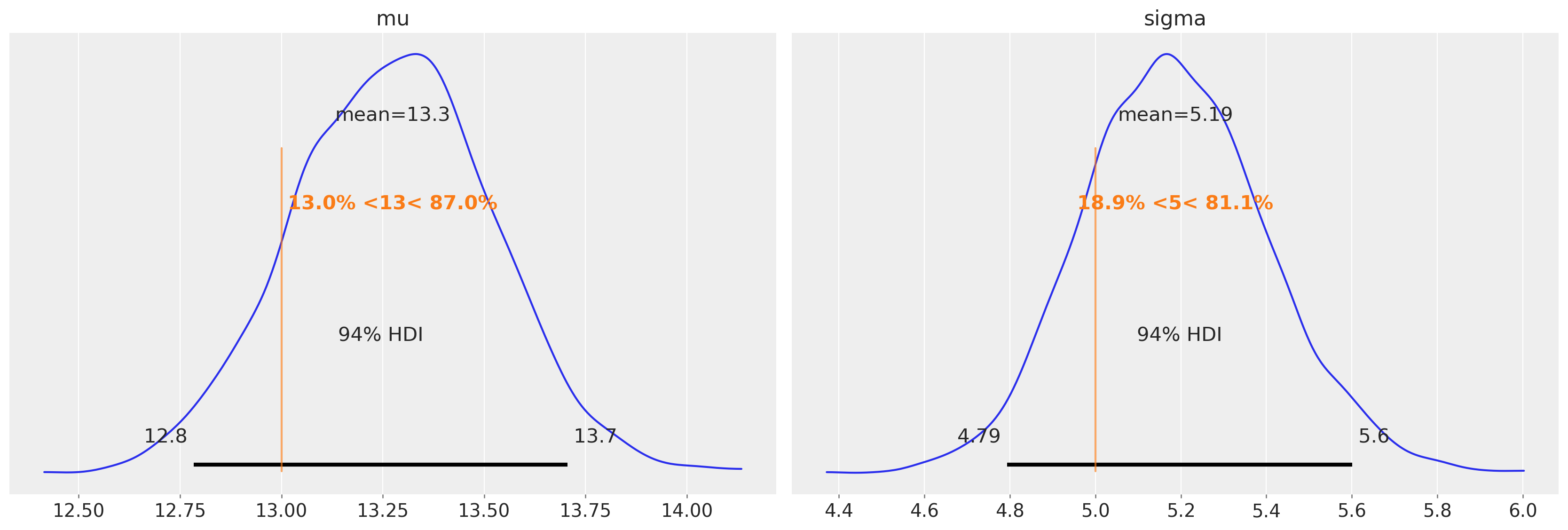
We can see that the bias in the estimates of the mean and variance (present in the uncensored model) have been largely removed.

Model 2 - Unimputed Censored Model of Censored Data

Here we can make use of pm.Censored.

with pm.Model() as unimputed_censored_model:
    mu = pm.Normal("mu", mu=0.0, sigma=(high - low) / 2.0)
    sigma = pm.HalfNormal("sigma", sigma=(high - low) / 2.0)
    y_latent = pm.Normal.dist(mu=mu, sigma=sigma)
    obs = pm.Censored("obs", y_latent, lower=low, upper=high, observed=censored)

Sampling

with unimputed_censored_model:
    idata = pm.sample()

az.plot_posterior(idata, var_names=["mu", "sigma"], ref_val=[true_mu, true_sigma], round_to=3);

Auto-assigning NUTS sampler...
Initializing NUTS using jitter+adapt_diag...
Multiprocess sampling (4 chains in 4 jobs)
NUTS: [mu, sigma]

100.00% [8000/8000 00:04<00:00 Sampling 4 chains, 0 divergences]

Sampling 4 chains for 1_000 tune and 1_000 draw iterations (4_000 + 4_000 draws total) took 5 seconds.

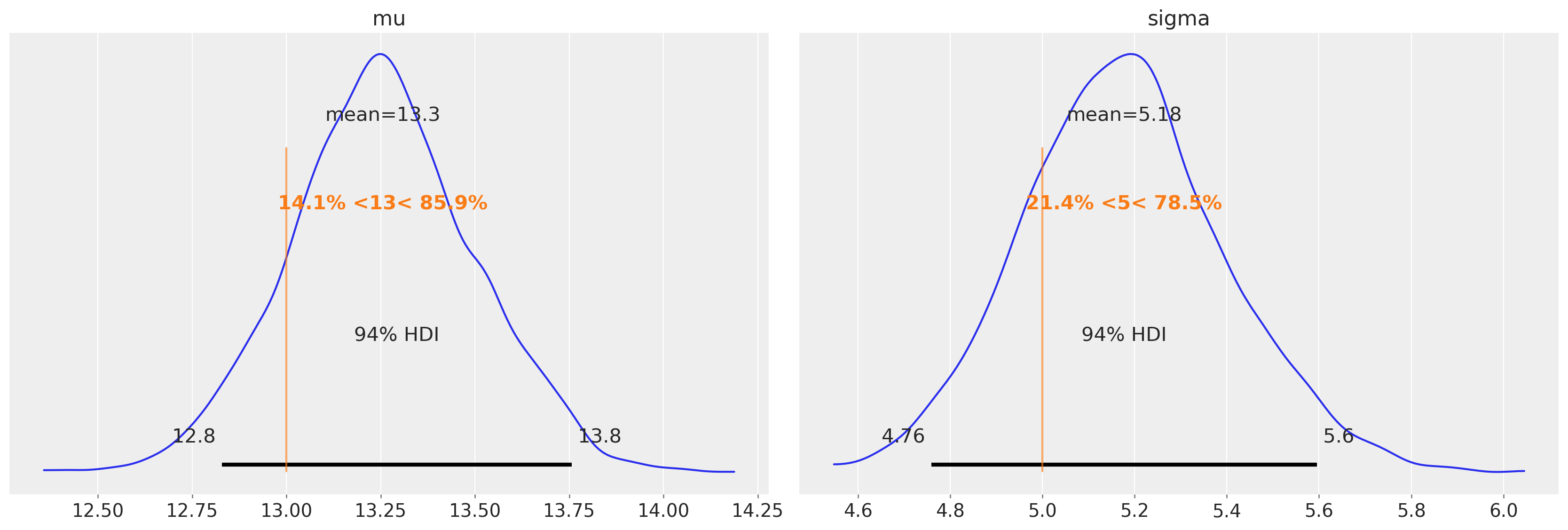
Again, the bias in the estimates of the mean and variance (present in the uncensored model) have been largely removed.

Discussion

As we can see, both censored models appear to capture the mean and variance of the underlying distribution as well as the uncensored model! In addition, the imputed censored model is capable of generating data sets of censored values (sample from the posteriors of left_censored and right_censored to generate them), while the unimputed censored model scales much better with more censored data, and converges faster.

Authors

• Originally authored by Luis Mario Domenzain on Mar 7, 2017.

• Updated by George Ho on Jul 14, 2018.

• Updated by Benjamin Vincent in May 2021.

• Updated by Benjamin Vincent in May 2022 to PyMC v4.

Watermark

%load_ext watermark
%watermark -n -u -v -iv -w -p pytensor,aeppl

Last updated: Tue Jan 17 2023

Python implementation: CPython
Python version       : 3.11.0
IPython version      : 8.8.0

pytensor: 2.9.1
aeppl   : not installed

seaborn   : 0.12.2
pymc      : 5.0.1+42.g99dd7158
arviz     : 0.14.0
matplotlib: 3.6.2
sys       : 3.11.0 | packaged by conda-forge | (main, Oct 25 2022, 06:24:40) [GCC 10.4.0]
numpy     : 1.24.1

Watermark: 2.3.1

License notice

All the notebooks in this example gallery are provided under the MIT License which allows modification, and redistribution for any use provided the copyright and license notices are preserved.

Citing PyMC examples

To cite this notebook, use the DOI provided by Zenodo for the pymc-examples repository.

Important

Many notebooks are adapted from other sources: blogs, books… In such cases you should cite the original source as well.

Also remember to cite the relevant libraries used by your code.

Here is an citation template in bibtex:

@incollection{citekey,
  author    = "<notebook authors, see above>",
  title     = "<notebook title>",
  editor    = "PyMC Team",
  booktitle = "PyMC examples",
  doi       = "10.5281/zenodo.5654871"
}

which once rendered could look like: