Marginalized Gaussian Mixture Model

import arviz as az
import numpy as np
import pymc3 as pm
import seaborn as sns

from matplotlib import pyplot as plt

print(f"Running on PyMC3 v{pm.__version__}")

Running on PyMC3 v3.11.2

%config InlineBackend.figure_format = 'retina'
RANDOM_SEED = 8927
rng = np.random.default_rng(RANDOM_SEED)
az.style.use("arviz-darkgrid")

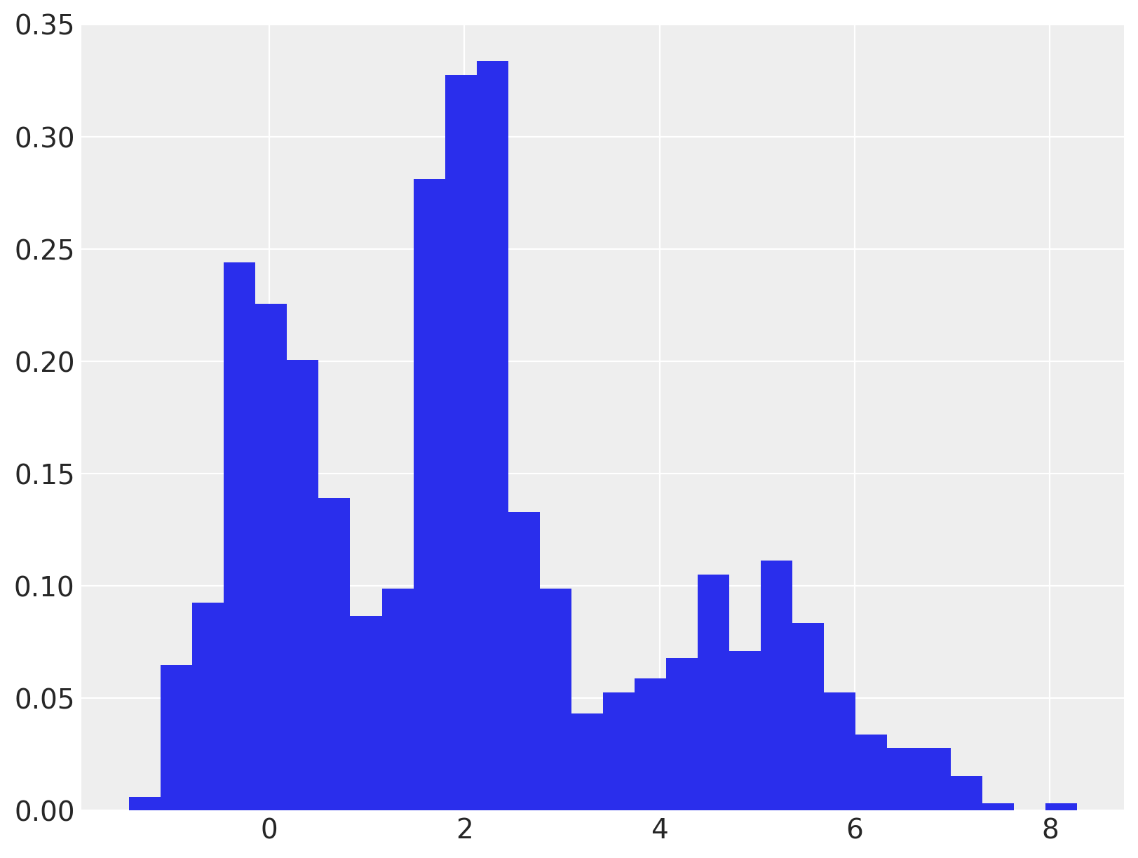
Gaussian mixtures are a flexible class of models for data that exhibits subpopulation heterogeneity. A toy example of such a data set is shown below.

N = 1000

W = np.array([0.35, 0.4, 0.25])

MU = np.array([0.0, 2.0, 5.0])
SIGMA = np.array([0.5, 0.5, 1.0])

component = rng.choice(MU.size, size=N, p=W)
x = rng.normal(MU[component], SIGMA[component], size=N)

fig, ax = plt.subplots(figsize=(8, 6))

ax.hist(x, bins=30, density=True, lw=0);

A natural parameterization of the Gaussian mixture model is as the latent variable model

\[\begin{split} \begin{align*} \mu_1, \ldots, \mu_K & \sim N(0, \sigma^2) \\ \tau_1, \ldots, \tau_K & \sim \textrm{Gamma}(a, b) \\ \boldsymbol{w} & \sim \textrm{Dir}(\boldsymbol{\alpha}) \\ z\ |\ \boldsymbol{w} & \sim \textrm{Cat}(\boldsymbol{w}) \\ x\ |\ z & \sim N(\mu_z, \tau^{-1}_z). \end{align*} \end{split}\]

An implementation of this parameterization in PyMC3 is available at Gaussian Mixture Model. A drawback of this parameterization is that is posterior relies on sampling the discrete latent variable \(z\). This reliance can cause slow mixing and ineffective exploration of the tails of the distribution.

An alternative, equivalent parameterization that addresses these problems is to marginalize over \(z\). The marginalized model is

\[\begin{split} \begin{align*} \mu_1, \ldots, \mu_K & \sim N(0, \sigma^2) \\ \tau_1, \ldots, \tau_K & \sim \textrm{Gamma}(a, b) \\ \boldsymbol{w} & \sim \textrm{Dir}(\boldsymbol{\alpha}) \\ f(x\ |\ \boldsymbol{w}) & = \sum_{i = 1}^K w_i\ N(x\ |\ \mu_i, \tau^{-1}_i), \end{align*} \end{split}\]

where

\[N(x\ |\ \mu, \sigma^2) = \frac{1}{\sqrt{2 \pi} \sigma} \exp\left(-\frac{1}{2 \sigma^2} (x - \mu)^2\right)\]

is the probability density function of the normal distribution.

Marginalizing \(z\) out of the model generally leads to faster mixing and better exploration of the tails of the posterior distribution. Marginalization over discrete parameters is a common trick in the Stan community, since Stan does not support sampling from discrete distributions. For further details on marginalization and several worked examples, see the Stan User’s Guide and Reference Manual.

PyMC3 supports marginalized Gaussian mixture models through its NormalMixture class. (It also supports marginalized general mixture models through its Mixture class) Below we specify and fit a marginalized Gaussian mixture model to this data in PyMC3.

with pm.Model(coords={"cluster": np.arange(len(W)), "obs_id": np.arange(N)}) as model:
    w = pm.Dirichlet("w", np.ones_like(W))

    mu = pm.Normal(
        "mu",
        np.zeros_like(W),
        1.0,
        dims="cluster",
        transform=pm.transforms.ordered,
        testval=[1, 2, 3],
    )
    tau = pm.Gamma("tau", 1.0, 1.0, dims="cluster")

    x_obs = pm.NormalMixture("x_obs", w, mu, tau=tau, observed=x, dims="obs_id")

with model:
    trace = pm.sample(5000, n_init=10000, tune=1000, return_inferencedata=True)

    # sample posterior predictive samples
    ppc_trace = pm.sample_posterior_predictive(trace, var_names=["x_obs"], keep_size=True)

trace.add_groups(posterior_predictive=ppc_trace)

Auto-assigning NUTS sampler...
Initializing NUTS using jitter+adapt_diag...
Multiprocess sampling (4 chains in 4 jobs)
NUTS: [tau, mu, w]

100.00% [24000/24000 00:27<00:00 Sampling 4 chains, 0 divergences]

Sampling 4 chains for 1_000 tune and 5_000 draw iterations (4_000 + 20_000 draws total) took 28 seconds.

0, dim: obs_id, 1000 =? 1000

100.00% [20000/20000 11:34<00:00]

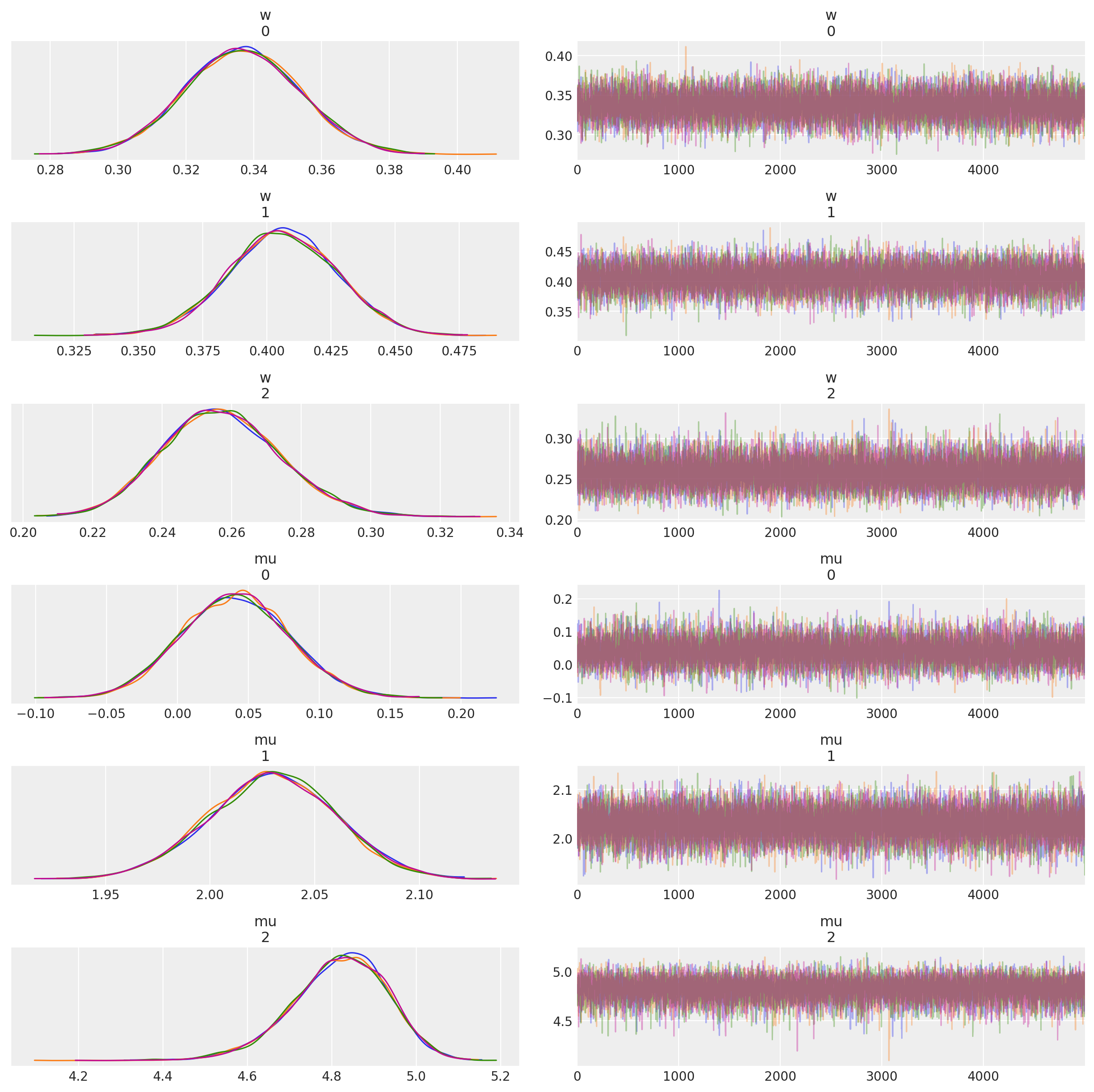
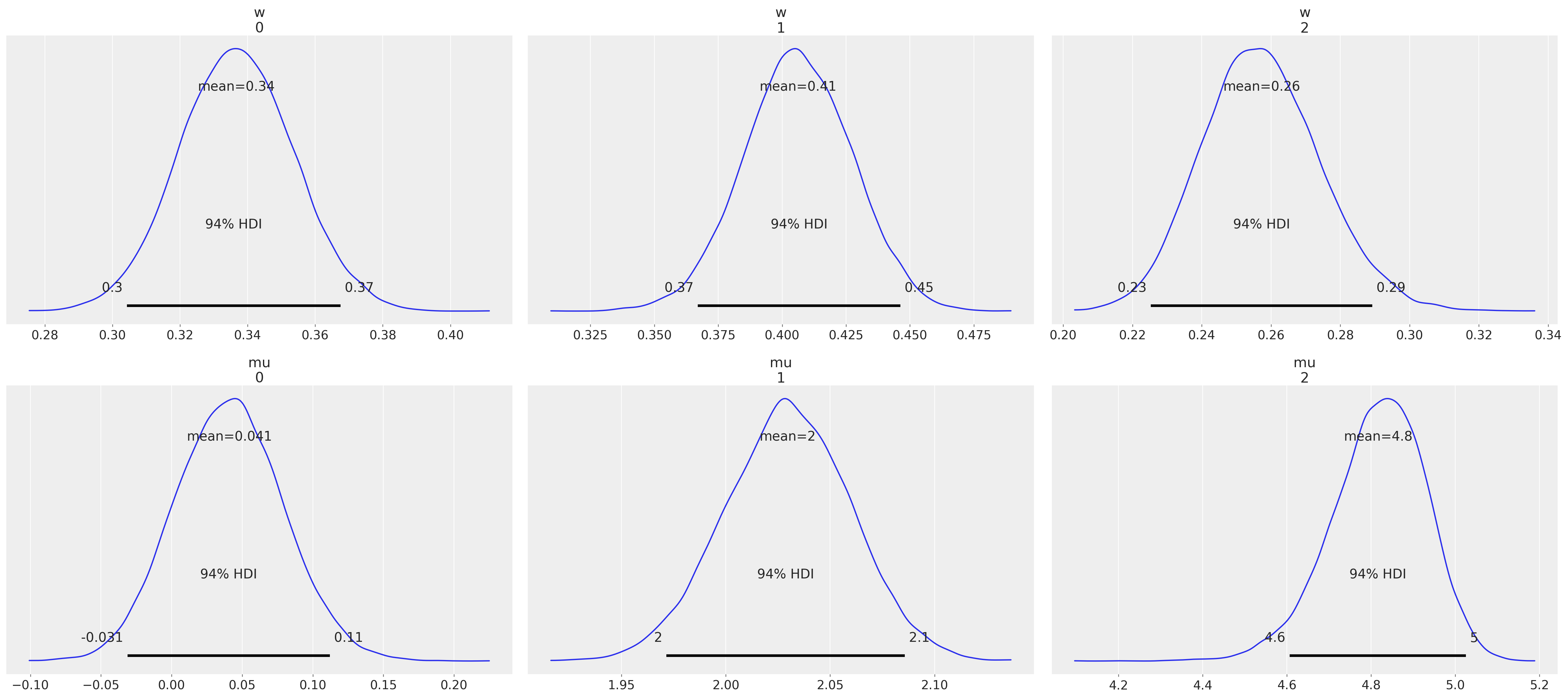
We see in the following plot that the posterior distribution on the weights and the component means has captured the true value quite well.

az.plot_trace(trace, var_names=["w", "mu"], compact=False);

az.plot_posterior(trace, var_names=["w", "mu"]);

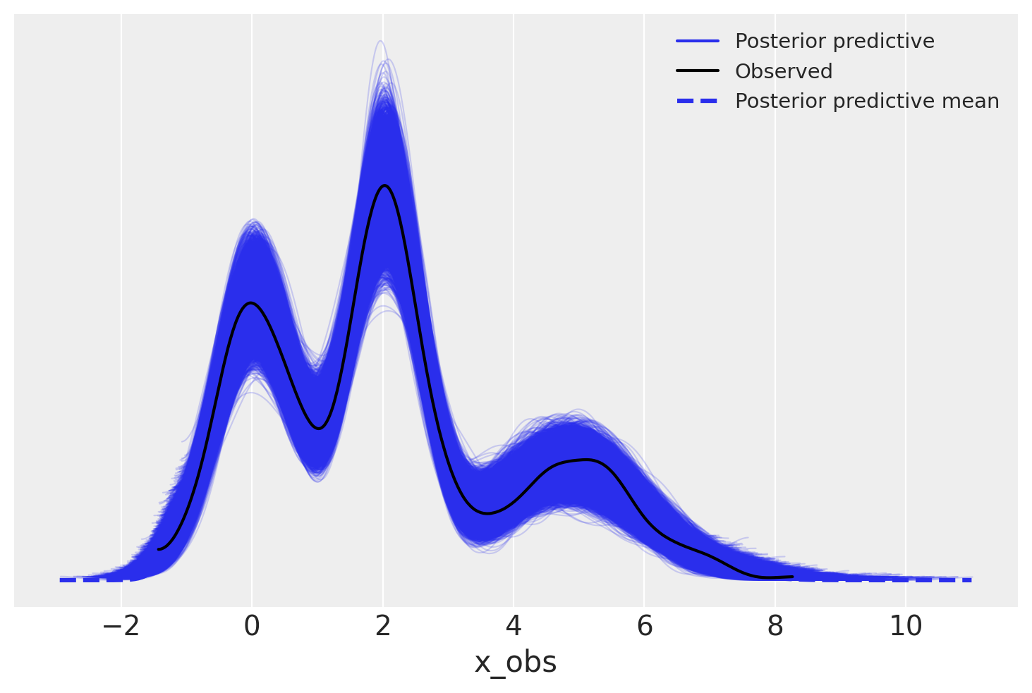
We see that the posterior predictive samples have a distribution quite close to that of the observed data.

az.plot_ppc(trace);

Author: Austin Rochford

Watermark

%load_ext watermark
%watermark -n -u -v -iv -w -p theano,xarray

Last updated: Mon Aug 30 2021

Python implementation: CPython
Python version       : 3.8.10
IPython version      : 7.25.0

theano: 1.1.2
xarray: 0.17.0

matplotlib: 3.3.4
numpy     : 1.21.0
seaborn   : 0.11.1
pymc3     : 3.11.2
arviz     : 0.11.2

Watermark: 2.2.0