


Gaussian Mixture Model#
A mixture model allows us to make inferences about the component contributors to a distribution of data. More specifically, a Gaussian Mixture Model allows us to make inferences about the means and standard deviations of a specified number of underlying component Gaussian distributions.
This could be useful in a number of ways. For example, we may be interested in simply describing a complex distribution parametrically (i.e. a mixture distribution). Alternatively, we may be interested in classification where we seek to probabilistically classify which of a number of classes a particular observation is from.
import arviz as az
import matplotlib.pyplot as plt
import numpy as np
import pandas as pd
import pymc as pm

from scipy.stats import norm
from xarray_einstats.stats import XrContinuousRV
%config InlineBackend.figure_format = 'retina'
RANDOM_SEED = 8927
rng = np.random.default_rng(RANDOM_SEED)
az.style.use("arviz-darkgrid")
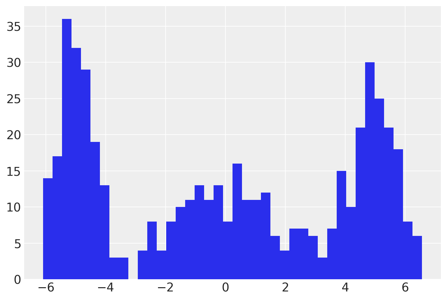
First we generate some simulated observations.
In the PyMC model, we will estimate one \(\mu\) and one \(\sigma\) for each of the 3 clusters. Writing a Gaussian Mixture Model is very easy with the pm.NormalMixture distribution.
with pm.Model(coords={"cluster": range(k)}) as model:
    μ = pm.Normal(
        "μ",
        mu=0,
        sigma=5,
        transform=pm.distributions.transforms.univariate_ordered,
        initval=[-4, 0, 4],
        dims="cluster",
    )
    σ = pm.HalfNormal("σ", sigma=1, dims="cluster")
    weights = pm.Dirichlet("w", np.ones(k), dims="cluster")
    pm.NormalMixture("x", w=weights, mu=μ, sigma=σ, observed=x)

pm.model_to_graphviz(model)

with model:
    idata = pm.sample()
Auto-assigning NUTS sampler...
Initializing NUTS using jitter+adapt_diag...
Multiprocess sampling (4 chains in 4 jobs)
NUTS: [μ, σ, w]
Sampling 4 chains for 1_000 tune and 1_000 draw iterations (4_000 + 4_000 draws total) took 4 seconds.
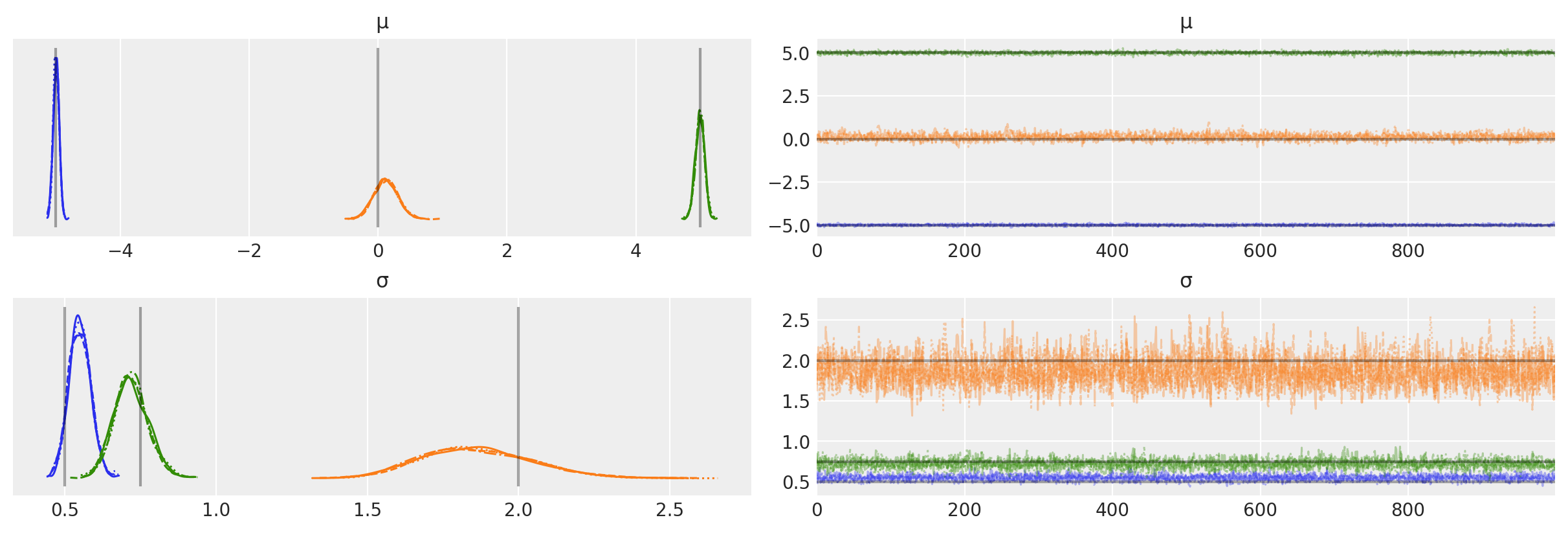
We can also plot the trace to check the nature of the MCMC chains, and compare to the ground truth values.
az.plot_trace(idata, var_names=["μ", "σ"], lines=[("μ", {}, [centers]), ("σ", {}, [sds])]);
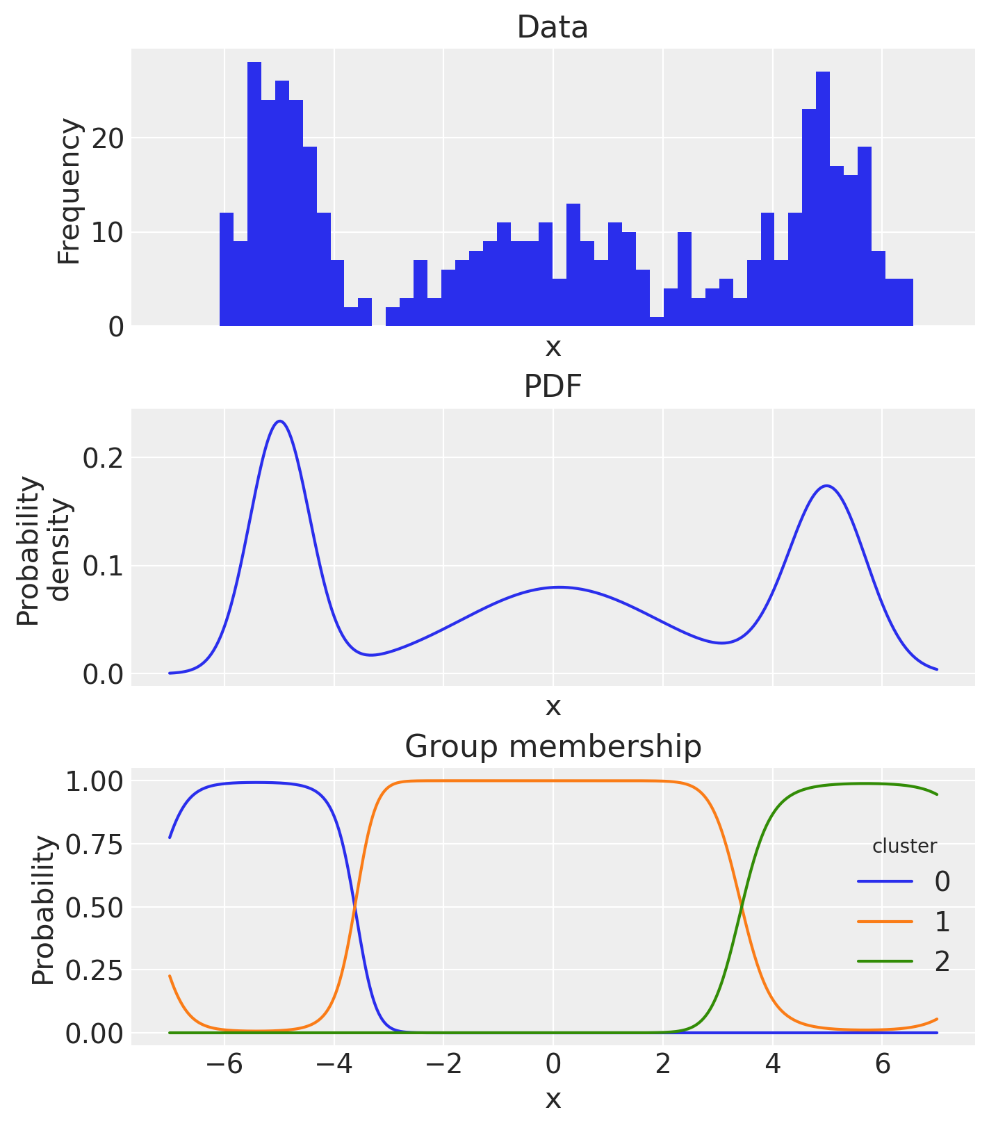
And if we wanted, we could calculate the probability density function and examine the estimated group membership probabilities, based on the posterior mean estimates.
xi = np.linspace(-7, 7, 500)
post = idata.posterior
pdf_components = XrContinuousRV(norm, post["μ"], post["σ"]).pdf(xi) * post["w"]
pdf = pdf_components.sum("cluster")

fig, ax = plt.subplots(3, 1, figsize=(7, 8), sharex=True)
# empirical histogram
ax[0].hist(x, 50)
ax[0].set(title="Data", xlabel="x", ylabel="Frequency")
# pdf
pdf_components.mean(dim=["chain", "draw"]).sum("cluster").plot.line(ax=ax[1])
ax[1].set(title="PDF", xlabel="x", ylabel="Probability\ndensity")
# plot group membership probabilities
(pdf_components / pdf).mean(dim=["chain", "draw"]).plot.line(hue="cluster", ax=ax[2])
ax[2].set(title="Group membership", xlabel="x", ylabel="Probability");
Watermark#
%load_ext watermark
%watermark -n -u -v -iv -w -p pytensor,aeppl,xarray,xarray_einstats
Last updated: Wed Feb 01 2023

Python implementation: CPython
Python version       : 3.11.0
IPython version      : 8.9.0

pytensor       : 2.8.11
aeppl          : not installed
xarray         : 2023.1.0
xarray_einstats: 0.5.1

pymc      : 5.0.1
arviz     : 0.14.0
numpy     : 1.24.1
pandas    : 1.5.3
matplotlib: 3.6.3

Watermark: 2.3.1
License notice#
All the notebooks in this example gallery are provided under the MIT License which allows modification, and redistribution for any use provided the copyright and license notices are preserved.
Citing PyMC examples#
To cite this notebook, use the DOI provided by Zenodo for the pymc-examples repository.
Important
Many notebooks are adapted from other sources: blogs, books… In such cases you should cite the original source as well.
Also remember to cite the relevant libraries used by your code.
Here is an citation template in bibtex:
@incollection{citekey,
  author    = "<notebook authors, see above>",
  title     = "<notebook title>",
  editor    = "PyMC Team",
  booktitle = "PyMC examples",
  doi       = "10.5281/zenodo.5654871"
}
which once rendered could look like: