


How to wrap a JAX function for use in PyMC#
import arviz as az
import matplotlib.pyplot as plt
import numpy as np
import pymc as pm
import pytensor
import pytensor.tensor as pt

from pytensor.graph import Apply, Op
RANDOM_SEED = 104109109
rng = np.random.default_rng(RANDOM_SEED)
az.style.use("arviz-darkgrid")
Attention
This notebook uses libraries that are not PyMC dependencies and therefore need to be installed specifically to run this notebook. Open the dropdown below for extra guidance.
Extra dependencies install instructions
In order to run this notebook (either locally or on binder) you won’t only need a working PyMC installation with all optional dependencies, but also to install some extra dependencies. For advise on installing PyMC itself, please refer to Installation
You can install these dependencies with your preferred package manager, we provide as an example the pip and conda commands below.
$ pip install jax numpyro
Note that if you want (or need) to install the packages from inside the notebook instead of the command line, you can install the packages by running a variation of the pip command:
import sys
!{sys.executable} -m pip install jax numpyro
You should not run !pip install as it might install the package in a different
environment and not be available from the Jupyter notebook even if installed.
Another alternative is using conda instead:
$ conda install jax numpyro
when installing scientific python packages with conda, we recommend using conda forge
import jax
import jax.numpy as jnp
import jax.scipy as jsp
import pymc.sampling_jax

from pytensor.link.jax.dispatch import jax_funcify
/home/ricardo/miniconda3/envs/pymc-examples/lib/python3.10/site-packages/pytensor/link/jax/dispatch.py:87: UserWarning: JAX omnistaging couldn't be disabled: Disabling of omnistaging is no longer supported in JAX version 0.2.12 and higher: see https://github.com/google/jax/blob/main/design_notes/omnistaging.md.
  warnings.warn(f"JAX omnistaging couldn't be disabled: {e}")
/home/ricardo/Documents/Projects/pymc/pymc/sampling_jax.py:36: UserWarning: This module is experimental.
  warnings.warn("This module is experimental.")
Intro: PyTensor and its backends#
PyMC uses the PyTensor library to create and manipulate probabilistic graphs. PyTensor is backend-agnostic, meaning it can make use of functions written in different languages or frameworks, including pure Python, NumPy, C, Cython, Numba, and JAX.
All that is needed is to encapsulate such function in a PyTensor Op, which enforces a specific API regarding how inputs and outputs of pure “operations” should be handled. It also implements methods for optional extra functionality like symbolic shape inference and automatic differentiation. This is well covered in the PyTensor Op documentation and in our Using a “black box” likelihood function pymc-example.
More recently, PyTensor became capable of compiling directly to some of these languages/frameworks, meaning that we can convert a complete PyTensor graph into a JAX or NUMBA jitted function, whereas traditionally they could only be converted to Python or C.
This has some interesting uses, such as sampling models defined in PyMC with pure JAX samplers, like those implemented in NumPyro or BlackJax.
This notebook illustrates how we can implement a new PyTensor Op that wraps a JAX function.
Outline#
We start in a similar path as that taken in the Using a “black box” likelihood function, which wraps a NumPy function in a PyTensor
Op, this time wrapping a JAX jitted function instead.We then enable PyTensor to “unwrap” the just wrapped JAX function, so that the whole graph can be compiled to JAX. We make use of this to sample our PyMC model via the JAX NumPyro NUTS sampler.
A motivating example: marginal HMM#
For illustration purposes, we will simulate data following a simple Hidden Markov Model (HMM), with 3 possible latent states \(S \in \{0, 1, 2\}\) and normal emission likelihood.
Our HMM will have a fixed Categorical probability \(P\) of switching across states, which depends only on the last state
To complete our model, we assume a fixed probability \(P_{t0}\) for each possible initial state \(S_{t0}\),
Simulating data#
Let’s generate data according to this model! The first step is to set some values for the parameters in our model
# Emission signal and noise parameters
emission_signal_true = 1.15
emission_noise_true = 0.15

p_initial_state_true = np.array([0.9, 0.09, 0.01])

# Probability of switching from state_t to state_t+1
p_transition_true = np.array(
    [
        #    0,   1,   2
        [0.9, 0.09, 0.01],  # 0
        [0.1, 0.8, 0.1],  # 1
        [0.2, 0.1, 0.7],  # 2
    ]
)

# Confirm that we have defined valid probabilities
assert np.isclose(np.sum(p_initial_state_true), 1)
assert np.allclose(np.sum(p_transition_true, axis=-1), 1)
# Let's compute the log of the probalitiy transition matrix for later use
with np.errstate(divide="ignore"):
    logp_initial_state_true = np.log(p_initial_state_true)
    logp_transition_true = np.log(p_transition_true)

logp_initial_state_true, logp_transition_true
(array([-0.10536052, -2.40794561, -4.60517019]),
 array([[-0.10536052, -2.40794561, -4.60517019],
        [-2.30258509, -0.22314355, -2.30258509],
        [-1.60943791, -2.30258509, -0.35667494]]))
# We will observe 70 HMM processes, each with a total of 50 steps
n_obs = 70
n_steps = 50
We write a helper function to generate a single HMM process and create our simulated data
def simulate_hmm(p_initial_state, p_transition, emission_signal, emission_noise, n_steps, rng):
    """Generate hidden state and emission from our HMM model."""

    possible_states = np.array([0, 1, 2])

    hidden_states = []
    initial_state = rng.choice(possible_states, p=p_initial_state)
    hidden_states.append(initial_state)
    for step in range(n_steps):
        new_hidden_state = rng.choice(possible_states, p=p_transition[hidden_states[-1]])
        hidden_states.append(new_hidden_state)
    hidden_states = np.array(hidden_states)

    emissions = rng.normal(
        (hidden_states + 1) * emission_signal,
        emission_noise,
    )

    return hidden_states, emissions
single_hmm_hidden_state, single_hmm_emission = simulate_hmm(
    p_initial_state_true,
    p_transition_true,
    emission_signal_true,
    emission_noise_true,
    n_steps,
    rng,
)
print(single_hmm_hidden_state)
print(np.round(single_hmm_emission, 2))
[0 0 0 0 0 0 1 1 1 1 1 1 0 0 0 0 0 1 1 1 1 1 1 1 1 1 1 1 1 1 1 1 1 1 2 2 1
 1 1 0 0 0 0 0 0 0 0 0 0 0 0]
[1.34 0.79 1.07 1.25 1.33 0.98 1.97 2.45 2.21 2.19 2.21 2.15 1.24 1.16
 0.78 1.18 1.34 2.21 2.44 2.14 2.15 2.38 2.27 2.33 2.26 2.37 2.45 2.36
 2.35 2.32 2.36 2.21 2.27 2.32 3.68 3.32 2.39 2.14 1.99 1.32 1.15 1.31
 1.25 1.17 1.06 0.91 0.88 1.17 1.   1.01 0.87]
hidden_state_true = []
emission_observed = []

for i in range(n_obs):
    hidden_state, emission = simulate_hmm(
        p_initial_state_true,
        p_transition_true,
        emission_signal_true,
        emission_noise_true,
        n_steps,
        rng,
    )
    hidden_state_true.append(hidden_state)
    emission_observed.append(emission)

hidden_state = np.array(hidden_state_true)
emission_observed = np.array(emission_observed)
fig, ax = plt.subplots(2, 1, figsize=(8, 6), sharex=True)
# Plot first five hmm processes
for i in range(4):
    ax[0].plot(hidden_state_true[i] + i * 0.02, color=f"C{i}", lw=2, alpha=0.4)
    ax[1].plot(emission_observed[i], color=f"C{i}", lw=2, alpha=0.4)
ax[0].set_yticks([0, 1, 2])
ax[0].set_ylabel("hidden state")
ax[1].set_ylabel("observed emmission")
ax[1].set_xlabel("step")
fig.suptitle("Simulated data");
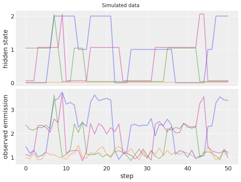
The figure above shows the hidden state and respective observed emission of our simulated data. Later, we will use this data to perform posterior inferences about the true model parameters.
Computing the marginal HMM likelihood using JAX#
We will write a JAX function to compute the likelihood of our HMM model, marginalizing over the hidden states. This allows for more efficient sampling of the remaining model parameters. To achieve this, we will use the well known forward algorithm, working on the log scale for numerical stability.
We will take advantage of JAX scan to obtain an efficient and differentiable log-likelihood, and the handy vmap to automatically vectorize this log-likelihood across multiple observed processes.
Our core JAX function computes the marginal log-likelihood of a single HMM process
def hmm_logp(
    emission_observed,
    emission_signal,
    emission_noise,
    logp_initial_state,
    logp_transition,
):
    """Compute the marginal log-likelihood of a single HMM process."""

    hidden_states = np.array([0, 1, 2])

    # Compute log-likelihood of observed emissions for each (step x possible hidden state)
    logp_emission = jsp.stats.norm.logpdf(
        emission_observed[:, None],
        (hidden_states + 1) * emission_signal,
        emission_noise,
    )

    # We use the forward_algorithm to compute log_alpha(x_t) = logp(x_t, y_1:t)
    log_alpha = logp_initial_state + logp_emission[0]
    log_alpha, _ = jax.lax.scan(
        f=lambda log_alpha_prev, logp_emission: (
            jsp.special.logsumexp(log_alpha_prev + logp_transition.T, axis=-1) + logp_emission,
            None,
        ),
        init=log_alpha,
        xs=logp_emission[1:],
    )

    return jsp.special.logsumexp(log_alpha)
Let’s test it with the true parameters and the first simulated HMM process
hmm_logp(
    emission_observed[0],
    emission_signal_true,
    emission_noise_true,
    logp_initial_state_true,
    logp_transition_true,
)
WARNING:absl:No GPU/TPU found, falling back to CPU. (Set TF_CPP_MIN_LOG_LEVEL=0 and rerun for more info.)
DeviceArray(-3.93533794, dtype=float64)
We now use vmap to vectorize the core function across multiple observations.
def vec_hmm_logp(*args):
    vmap = jax.vmap(
        hmm_logp,
        # Only the first argument, needs to be vectorized
        in_axes=(0, None, None, None, None),
    )
    # For simplicity we sum across all the HMM processes
    return jnp.sum(vmap(*args))


# We jit it for better performance!
jitted_vec_hmm_logp = jax.jit(vec_hmm_logp)
Passing a row matrix with only the first simulated HMM process should return the same result
jitted_vec_hmm_logp(
    emission_observed[0][None, :],
    emission_signal_true,
    emission_noise_true,
    logp_initial_state_true,
    logp_transition_true,
)
DeviceArray(-3.93533794, dtype=float64)
Our goal is, however, to compute the joint log-likelihood for all the simulated data
jitted_vec_hmm_logp(
    emission_observed,
    emission_signal_true,
    emission_noise_true,
    logp_initial_state_true,
    logp_transition_true,
)
DeviceArray(-37.00348857, dtype=float64)
We will also ask JAX to give us the function of the gradients with respect to each input. This will come in handy later.
jitted_vec_hmm_logp_grad = jax.jit(jax.grad(vec_hmm_logp, argnums=list(range(5))))
Let’s print out the gradient with respect to emission_signal. We will check this value is unchanged after we wrap our function in PyTensor.
jitted_vec_hmm_logp_grad(
    emission_observed,
    emission_signal_true,
    emission_noise_true,
    logp_initial_state_true,
    logp_transition_true,
)[1]
DeviceArray(-297.86490611, dtype=float64, weak_type=True)
Wrapping the JAX function in PyTensor#
Now we are ready to wrap our JAX jitted function in a PyTensor Op, that we can then use in our PyMC models. We recommend you check PyTensor’s official Op documentation if you want to understand it in more detail.
In brief, we will inherit from Op and define the following methods:
make_node: Creates anApplynode that holds together the symbolic inputs and outputs of our operationperform: Python code that returns the evaluation of our operation, given concrete input valuesgrad: Returns a PyTensor symbolic graph that represents the gradient expression of an output cost wrt to its inputs
For the grad we will create a second Op that wraps our jitted grad version from above
class HMMLogpOp(Op):
    def make_node(
        self,
        emission_observed,
        emission_signal,
        emission_noise,
        logp_initial_state,
        logp_transition,
    ):
        # Convert our inputs to symbolic variables
        inputs = [
            pt.as_tensor_variable(emission_observed),
            pt.as_tensor_variable(emission_signal),
            pt.as_tensor_variable(emission_noise),
            pt.as_tensor_variable(logp_initial_state),
            pt.as_tensor_variable(logp_transition),
        ]
        # Define the type of the output returned by the wrapped JAX function
        outputs = [pt.dscalar()]
        return Apply(self, inputs, outputs)

    def perform(self, node, inputs, outputs):
        result = jitted_vec_hmm_logp(*inputs)
        # PyTensor raises an error if the dtype of the returned output is not
        # exactly the one expected from the Apply node (in this case
        # `dscalar`, which stands for float64 scalar), so we make sure
        # to convert to the expected dtype. To avoid unnecessary conversions
        # you should make sure the expected output defined in `make_node`
        # is already of the correct dtype
        outputs[0][0] = np.asarray(result, dtype=node.outputs[0].dtype)

    def grad(self, inputs, output_gradients):
        (
            grad_wrt_emission_obsered,
            grad_wrt_emission_signal,
            grad_wrt_emission_noise,
            grad_wrt_logp_initial_state,
            grad_wrt_logp_transition,
        ) = hmm_logp_grad_op(*inputs)
        # If there are inputs for which the gradients will never be needed or cannot
        # be computed, `pytensor.gradient.grad_not_implemented` should  be used as the
        # output gradient for that input.
        output_gradient = output_gradients[0]
        return [
            output_gradient * grad_wrt_emission_obsered,
            output_gradient * grad_wrt_emission_signal,
            output_gradient * grad_wrt_emission_noise,
            output_gradient * grad_wrt_logp_initial_state,
            output_gradient * grad_wrt_logp_transition,
        ]


class HMMLogpGradOp(Op):
    def make_node(
        self,
        emission_observed,
        emission_signal,
        emission_noise,
        logp_initial_state,
        logp_transition,
    ):
        inputs = [
            pt.as_tensor_variable(emission_observed),
            pt.as_tensor_variable(emission_signal),
            pt.as_tensor_variable(emission_noise),
            pt.as_tensor_variable(logp_initial_state),
            pt.as_tensor_variable(logp_transition),
        ]
        # This `Op` will return one gradient per input. For simplicity, we assume
        # each output is of the same type as the input. In practice, you should use
        # the exact dtype to avoid overhead when saving the results of the computation
        # in `perform`
        outputs = [inp.type() for inp in inputs]
        return Apply(self, inputs, outputs)

    def perform(self, node, inputs, outputs):
        (
            grad_wrt_emission_obsered_result,
            grad_wrt_emission_signal_result,
            grad_wrt_emission_noise_result,
            grad_wrt_logp_initial_state_result,
            grad_wrt_logp_transition_result,
        ) = jitted_vec_hmm_logp_grad(*inputs)
        outputs[0][0] = np.asarray(grad_wrt_emission_obsered_result, dtype=node.outputs[0].dtype)
        outputs[1][0] = np.asarray(grad_wrt_emission_signal_result, dtype=node.outputs[1].dtype)
        outputs[2][0] = np.asarray(grad_wrt_emission_noise_result, dtype=node.outputs[2].dtype)
        outputs[3][0] = np.asarray(grad_wrt_logp_initial_state_result, dtype=node.outputs[3].dtype)
        outputs[4][0] = np.asarray(grad_wrt_logp_transition_result, dtype=node.outputs[4].dtype)


# Initialize our `Op`s
hmm_logp_op = HMMLogpOp()
hmm_logp_grad_op = HMMLogpGradOp()
We recommend using the debug helper eval method to confirm we specified everything correctly. We should get the same outputs as before:
hmm_logp_op(
    emission_observed,
    emission_signal_true,
    emission_noise_true,
    logp_initial_state_true,
    logp_transition_true,
).eval()
array(-37.00348857)
hmm_logp_grad_op(
    emission_observed,
    emission_signal_true,
    emission_noise_true,
    logp_initial_state_true,
    logp_transition_true,
)[1].eval()
array(-297.86490611)
It’s also useful to check the gradient of our Op can be requested via the PyTensor grad interface:
# We define the symbolic `emission_signal` variable outside of the `Op`
# so that we can request the gradient wrt to it
emission_signal_variable = pt.as_tensor_variable(emission_signal_true)
x = hmm_logp_op(
    emission_observed,
    emission_signal_variable,
    emission_noise_true,
    logp_initial_state_true,
    logp_transition_true,
)
x_grad_wrt_emission_signal = pt.grad(x, wrt=emission_signal_variable)
x_grad_wrt_emission_signal.eval()
array(-297.86490611)
Sampling with PyMC#
We are now ready to make inferences about our HMM model with PyMC. We will define priors for each model parameter and use Potential to add the joint log-likelihood term to our model.
with pm.Model() as model:
    emission_signal = pm.Normal("emission_signal", 0, 1)
    emission_noise = pm.HalfNormal("emission_noise", 1)

    p_initial_state = pm.Dirichlet("p_initial_state", np.ones(3))
    logp_initial_state = pt.log(p_initial_state)

    p_transition = pm.Dirichlet("p_transition", np.ones(3), size=3)
    logp_transition = pt.log(p_transition)

    loglike = pm.Potential(
        "hmm_loglike",
        hmm_logp_op(
            emission_observed,
            emission_signal,
            emission_noise,
            logp_initial_state,
            logp_transition,
        ),
    )
pm.model_to_graphviz(model)

Before we start sampling, we check the logp of each variable at the model initial point. Bugs tend to manifest themselves in the form of nan or -inf for the initial probabilities.
initial_point = model.initial_point()
initial_point
{'emission_signal': array(0.),
 'emission_noise_log__': array(0.),
 'p_initial_state_simplex__': array([0., 0.]),
 'p_transition_simplex__': array([[0., 0.],
        [0., 0.],
        [0., 0.]])}
model.point_logps(initial_point)
{'emission_signal': -0.92,
 'emission_noise': -0.73,
 'p_initial_state': -1.5,
 'p_transition': -4.51,
 'hmm_loglike': -9812.67}
We are now ready to sample!
with model:
    idata = pm.sample(chains=2, cores=1)
Auto-assigning NUTS sampler...
INFO:pymc:Auto-assigning NUTS sampler...
Initializing NUTS using jitter+adapt_diag...
INFO:pymc:Initializing NUTS using jitter+adapt_diag...
/home/ricardo/Documents/Projects/pymc/pymc/pytensorf.py:1005: UserWarning: The parameter 'updates' of pytensor.function() expects an OrderedDict, got <class 'dict'>. Using a standard dictionary here results in non-deterministic behavior. You should use an OrderedDict if you are using Python 2.7 (collections.OrderedDict for older python), or use a list of (shared, update) pairs. Do not just convert your dictionary to this type before the call as the conversion will still be non-deterministic.
  pytensor_function = pytensor.function(
Sequential sampling (2 chains in 1 job)
INFO:pymc:Sequential sampling (2 chains in 1 job)
NUTS: [emission_signal, emission_noise, p_initial_state, p_transition]
INFO:pymc:NUTS: [emission_signal, emission_noise, p_initial_state, p_transition]
Sampling 2 chains for 1_000 tune and 1_000 draw iterations (2_000 + 2_000 draws total) took 109 seconds.
INFO:pymc:Sampling 2 chains for 1_000 tune and 1_000 draw iterations (2_000 + 2_000 draws total) took 109 seconds.
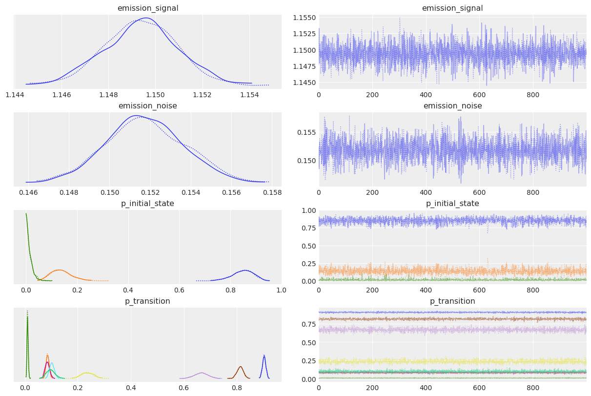
az.plot_trace(idata);
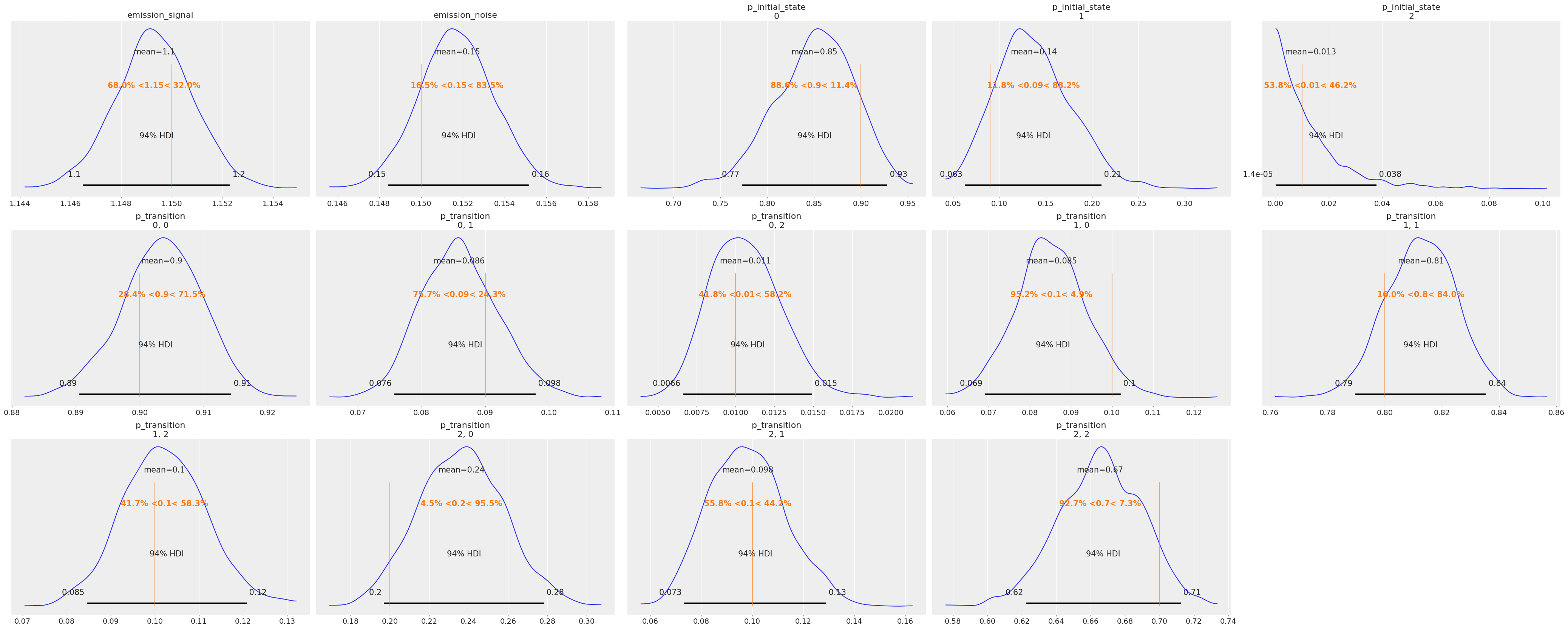
true_values = [
    emission_signal_true,
    emission_noise_true,
    *p_initial_state_true,
    *p_transition_true.ravel(),
]

az.plot_posterior(idata, ref_val=true_values, grid=(3, 5));
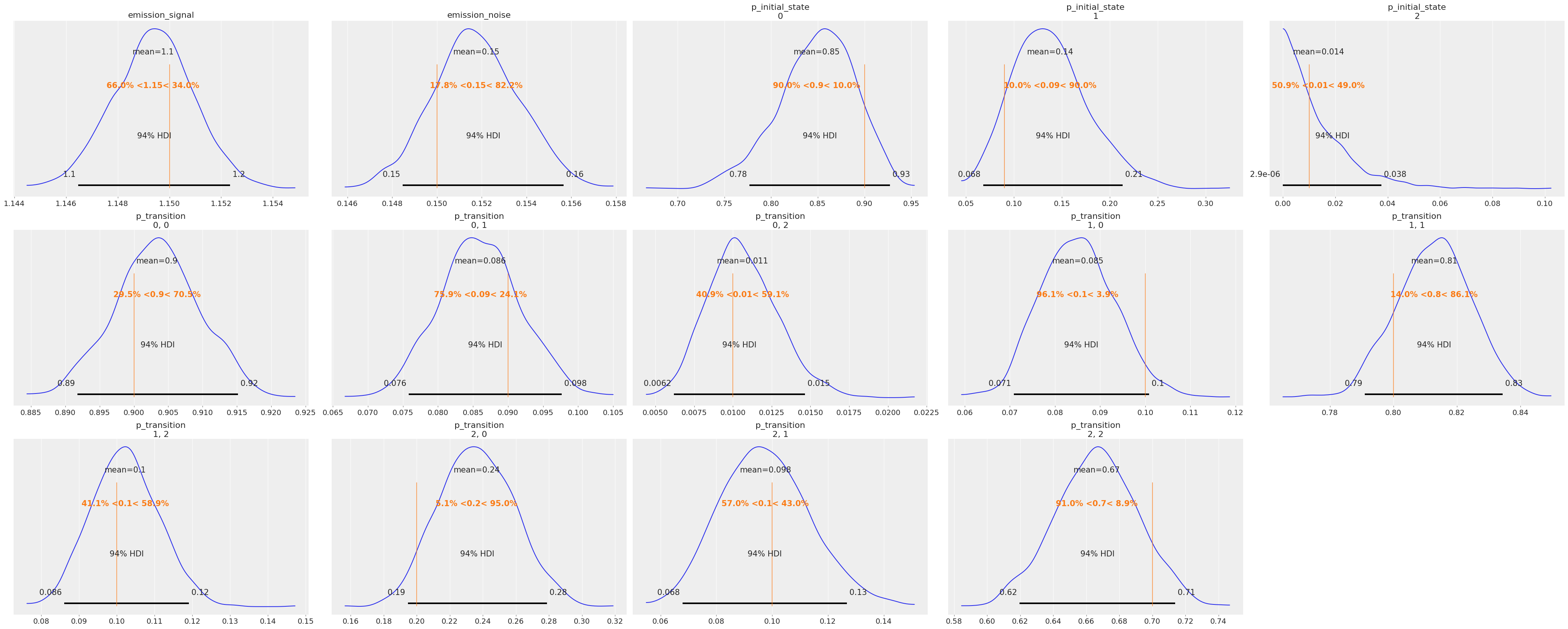
The posteriors look reasonably centered around the true values used to generate our data.
Unwrapping the wrapped JAX function#
As mentioned in the beginning, PyTensor can compile an entire graph to JAX. To do this, it needs to know how each Op in the graph can be converted to a JAX function. This can be done by dispatch with pytensor.link.jax.dispatch.jax_funcify(). Most of the default PyTensor Ops already have such a dispatch function, but we will need to add a new one for our custom HMMLogpOp, as PyTensor has never seen that before.
For that we need a function which returns (another) JAX function, that performs the same computation as in our perform method. Fortunately, we started exactly with such function, so this amounts to 3 short lines of code.
@jax_funcify.register(HMMLogpOp)
def hmm_logp_dispatch(op, **kwargs):
    return vec_hmm_logp
Note
We do not return the jitted function, so that the entire PyTensor graph can be jitted together after being converted to JAX.
For a better understanding of Op JAX conversions, we recommend reading PyTensor’s Adding JAX and Numba support for Ops guide.
We can test that our conversion function is working properly by compiling a pytensor.function() with mode="JAX":
out = hmm_logp_op(
    emission_observed,
    emission_signal_true,
    emission_noise_true,
    logp_initial_state_true,
    logp_transition_true,
)
jax_fn = pytensor.function(inputs=[], outputs=out, mode="JAX")
jax_fn()
DeviceArray(-37.00348857, dtype=float64)
We can also compile a JAX function that computes the log probability of each variable in our PyMC model, similar to point_logps(). We will use the helper method compile_fn().
model_logp_jax_fn = model.compile_fn(model.logp(sum=False), mode="JAX")
model_logp_jax_fn(initial_point)
[DeviceArray(-0.91893853, dtype=float64),
 DeviceArray(-0.72579135, dtype=float64),
 DeviceArray(-1.5040774, dtype=float64),
 DeviceArray([-1.5040774, -1.5040774, -1.5040774], dtype=float64),
 DeviceArray(-9812.66649064, dtype=float64)]
Note that we could have added an equally simple function to convert our HMMLogpGradOp, in case we wanted to convert PyTensor gradient graphs to JAX. In our case, we don’t need to do this because we will rely on JAX grad function (or more precisely, NumPyro will rely on it) to obtain these again from our compiled JAX function.
We include a short discussion at the end of this document, to help you better understand the trade-offs between working with PyTensor graphs vs JAX functions, and when you might want to use one or the other.
Sampling with NumPyro#
Now that we know our model logp can be entirely compiled to JAX, we can use the handy pymc.sampling_jax.sample_numpyro_nuts() to sample our model using the pure JAX sampler implemented in NumPyro.
with model:
    idata_numpyro = pm.sampling_jax.sample_numpyro_nuts(chains=2, progressbar=False)
/home/ricardo/miniconda3/envs/pymc-examples/lib/python3.10/site-packages/tqdm/auto.py:22: TqdmWarning: IProgress not found. Please update jupyter and ipywidgets. See https://ipywidgets.readthedocs.io/en/stable/user_install.html
  from .autonotebook import tqdm as notebook_tqdm
/home/ricardo/Documents/Projects/pymc/pymc/pytensorf.py:1005: UserWarning: The parameter 'updates' of pytensor.function() expects an OrderedDict, got <class 'dict'>. Using a standard dictionary here results in non-deterministic behavior. You should use an OrderedDict if you are using Python 2.7 (collections.OrderedDict for older python), or use a list of (shared, update) pairs. Do not just convert your dictionary to this type before the call as the conversion will still be non-deterministic.
  pytensor_function = pytensor.function(
Compiling...
Compilation time =  0:00:01.897853
Sampling...
Sampling time =  0:00:47.542330
Transforming variables...
Transformation time =  0:00:00.399051
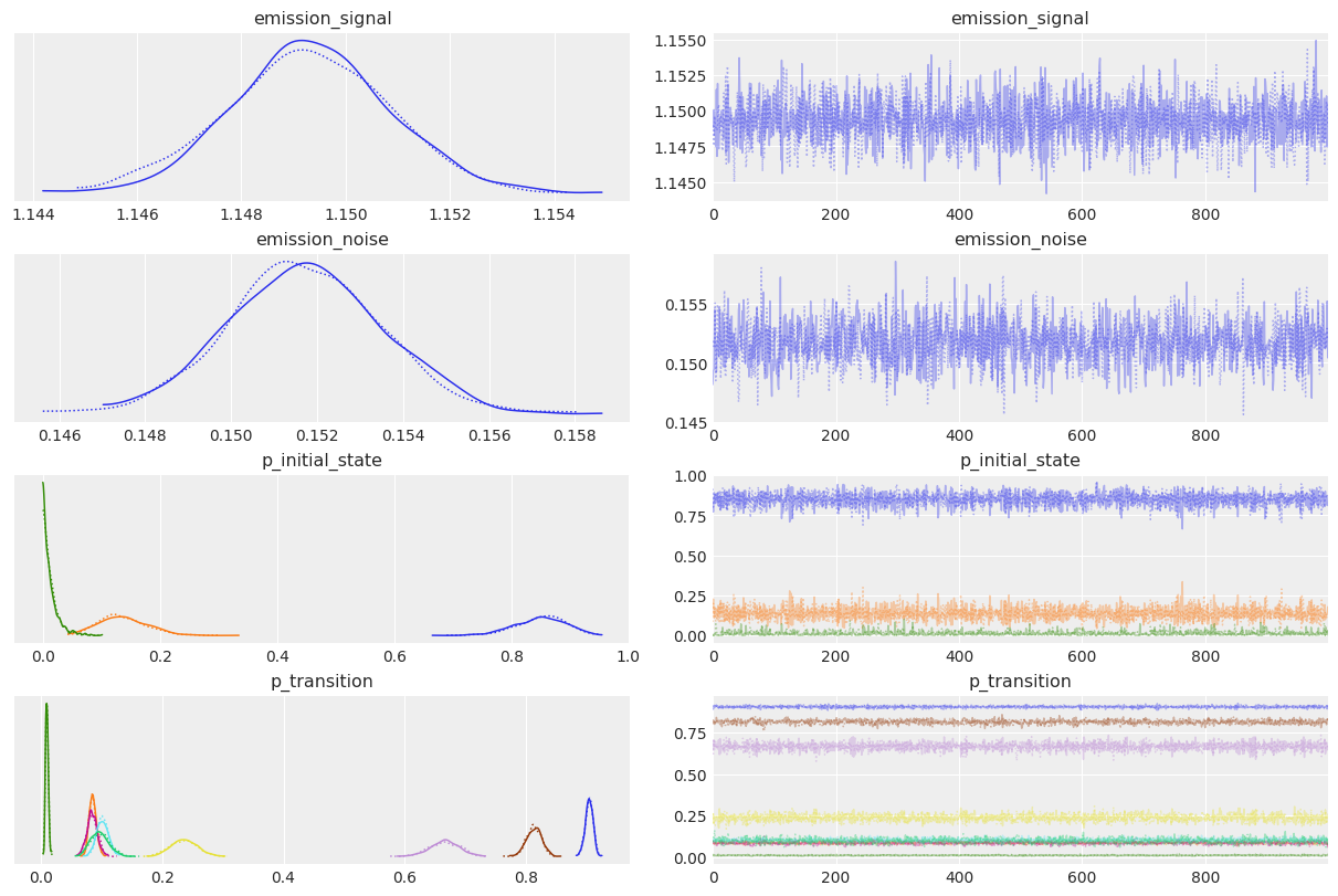
az.plot_trace(idata_numpyro);
az.plot_posterior(idata_numpyro, ref_val=true_values, grid=(3, 5));
As expected, sampling results look pretty similar!
Depending on the model and computer architecture you are using, a pure JAX sampler can provide considerable speedups.
Some brief notes on using PyTensor vs JAX#
When should you use JAX?#
As we have seen, it is pretty straightforward to interface between PyTensor graphs and JAX functions.
This can be very handy when you want to combine previously implemented JAX function with PyMC models. We used a marginalized HMM log-likelihood in this example, but the same strategy could be used to do Bayesian inference with Deep Neural Networks or Differential Equations, or pretty much any other functions implemented in JAX that can be used in the context of a Bayesian model.
It can also be worth it, if you need to make use of JAX’s unique features like vectorization, support for tree structures, or its fine-grained parallelization, and GPU and TPU capabilities.
When should you not use JAX?#
Like JAX, PyTensor has the goal of mimicking the NumPy and Scipy APIs, so that writing code in PyTensor should feel very similar to how code is written in those libraries.
There are, however, some of advantages to working with PyTensor:
PyTensor graphs are considerably easier to inspect and debug than JAX functions
PyTensor has clever optimization and stabilization routines that are not possible or implemented in JAX
PyTensor graphs can be easily manipulated after creation
Point 2 means your graphs are likely to perform better if written in PyTensor. In general you don’t have to worry about using specialized functions like log1p or logsumexp, as PyTensor will be able to detect the equivalent naive expressions and replace them by their specialized counterparts. Importantly, you still benefit from these optimizations when your graph is later compiled to JAX.
The catch is that PyTensor cannot reason about JAX functions, and by association Ops that wrap them. This means that the larger the portion of the graph is “hidden” inside a JAX function, the less a user will benefit from PyTensor’s rewrite and debugging abilities.
Point 3 is more important for library developers. It is the main reason why PyMC developers opted to use PyTensor (and before that, its predecessor Theano) as its backend. Many of the user-facing utilities provided by PyMC rely on the ability to easily parse and manipulate PyTensor graphs.
Bonus: Using a single Op that can compute its own gradients#
We had to create two Ops, one for the function we cared about and a separate one for its gradients. However, JAX provides a value_and_grad utility that can return both the value of a function and its gradients. We can do something similar and get away with a single Op if we are clever about it.
By doing this we can (potentially) save memory and reuse computation that is shared between the function and its gradients. This may be relevant when working with very large JAX functions.
Note that this is only useful if you are interested in taking gradients with respect to your Op using PyTensor. If your endgoal is to compile your graph to JAX, and only then take the gradients (as NumPyro does), then it’s better to use the first approach. You don’t even need to implement the grad method and associated Op in that case.
jitted_hmm_logp_value_and_grad = jax.jit(jax.value_and_grad(vec_hmm_logp, argnums=list(range(5))))
class HmmLogpValueGradOp(Op):
    # By default only show the first output, and "hide" the other ones
    default_output = 0

    def make_node(self, *inputs):
        inputs = [pt.as_tensor_variable(inp) for inp in inputs]
        # We now have one output for the function value, and one output for each gradient
        outputs = [pt.dscalar()] + [inp.type() for inp in inputs]
        return Apply(self, inputs, outputs)

    def perform(self, node, inputs, outputs):
        result, grad_results = jitted_hmm_logp_value_and_grad(*inputs)
        outputs[0][0] = np.asarray(result, dtype=node.outputs[0].dtype)
        for i, grad_result in enumerate(grad_results, start=1):
            outputs[i][0] = np.asarray(grad_result, dtype=node.outputs[i].dtype)

    def grad(self, inputs, output_gradients):
        # The `Op` computes its own gradients, so we call it again.
        value = self(*inputs)
        # We hid the gradient outputs by setting `default_update=0`, but we
        # can retrieve them anytime by accessing the `Apply` node via `value.owner`
        gradients = value.owner.outputs[1:]

        # Make sure the user is not trying to take the gradient with respect to
        # the gradient outputs! That would require computing the second order
        # gradients
        assert all(
            isinstance(g.type, pytensor.gradient.DisconnectedType) for g in output_gradients[1:]
        )

        return [output_gradients[0] * grad for grad in gradients]


hmm_logp_value_grad_op = HmmLogpValueGradOp()
We check again that we can take the gradient using PyTensor grad interface
emission_signal_variable = pt.as_tensor_variable(emission_signal_true)
# Only the first output is assigned to the variable `x`, due to `default_output=0`
x = hmm_logp_value_grad_op(
    emission_observed,
    emission_signal_variable,
    emission_noise_true,
    logp_initial_state_true,
    logp_transition_true,
)
pt.grad(x, emission_signal_variable).eval()
array(-297.86490611)
Watermark#
%load_ext watermark
%watermark -n -u -v -iv -w -p pytensor,aeppl,xarray
Last updated: Mon Apr 11 2022

Python implementation: CPython
Python version       : 3.10.2
IPython version      : 8.1.1

pytensor: 2.5.1
aeppl : 0.0.27
xarray: 2022.3.0

matplotlib: 3.5.1
jax       : 0.3.4
pytensor    : 2.5.1
arviz     : 0.12.0
pymc      : 4.0.0b6
numpy     : 1.22.3

Watermark: 2.3.0
License notice#
All the notebooks in this example gallery are provided under the MIT License which allows modification, and redistribution for any use provided the copyright and license notices are preserved.
Citing PyMC examples#
To cite this notebook, use the DOI provided by Zenodo for the pymc-examples repository.
Important
Many notebooks are adapted from other sources: blogs, books… In such cases you should cite the original source as well.
Also remember to cite the relevant libraries used by your code.
Here is an citation template in bibtex:
@incollection{citekey,
  author    = "<notebook authors, see above>",
  title     = "<notebook title>",
  editor    = "PyMC Team",
  booktitle = "PyMC examples",
  doi       = "10.5281/zenodo.5654871"
}
which once rendered could look like: