GLM: Poisson Regression#

This is a minimal reproducible example of Poisson regression to predict counts using dummy data.

This Notebook is basically an excuse to demo Poisson regression using PyMC, both manually and using bambi to demo interactions using the formulae library. We will create some dummy data, Poisson distributed according to a linear model, and try to recover the coefficients of that linear model through inference.

For more statistical detail see:

Basic info on Wikipedia
GLMs: Poisson regression, exposure, and overdispersion in Chapter 6.2 of ARM, Gelmann & Hill 2006
This worked example from ARM 6.2 by Clay Ford

This very basic model is inspired by a project by Ian Osvald, which is concerned with understanding the various effects of external environmental factors upon the allergic sneezing of a test subject.

#!pip install seaborn

import arviz as az
import bambi as bmb
import matplotlib.pyplot as plt
import numpy as np
import pandas as pd
import pymc as pm
import seaborn as sns

from formulae import design_matrices

RANDOM_SEED = 8927
rng = np.random.default_rng(RANDOM_SEED)

%config InlineBackend.figure_format = 'retina'
az.style.use("arviz-darkgrid")

Local Functions#

Generate Data#

This dummy dataset is created to emulate some data created as part of a study into quantified self, and the real data is more complicated than this. Ask Ian Osvald if you’d like to know more @ianozvald.

Assumptions:#

The subject sneezes N times per day, recorded as nsneeze (int)
The subject may or may not drink alcohol during that day, recorded as alcohol (boolean)
The subject may or may not take an antihistamine medication during that day, recorded as the negative action nomeds (boolean)
We postulate (probably incorrectly) that sneezing occurs at some baseline rate, which increases if an antihistamine is not taken, and further increased after alcohol is consumed.
The data is aggregated per day, to yield a total count of sneezes on that day, with a boolean flag for alcohol and antihistamine usage, with the big assumption that nsneezes have a direct causal relationship.

Create 4000 days of data: daily counts of sneezes which are Poisson distributed w.r.t alcohol consumption and antihistamine usage

# decide poisson theta values
theta_noalcohol_meds = 1  # no alcohol, took an antihist
theta_alcohol_meds = 3  # alcohol, took an antihist
theta_noalcohol_nomeds = 6  # no alcohol, no antihist
theta_alcohol_nomeds = 36  # alcohol, no antihist

# create samples
q = 1000
df = pd.DataFrame(
    {
        "nsneeze": np.concatenate(
            (
                rng.poisson(theta_noalcohol_meds, q),
                rng.poisson(theta_alcohol_meds, q),
                rng.poisson(theta_noalcohol_nomeds, q),
                rng.poisson(theta_alcohol_nomeds, q),
            )
        ),
        "alcohol": np.concatenate(
            (
                np.repeat(False, q),
                np.repeat(True, q),
                np.repeat(False, q),
                np.repeat(True, q),
            )
        ),
        "nomeds": np.concatenate(
            (
                np.repeat(False, q),
                np.repeat(False, q),
                np.repeat(True, q),
                np.repeat(True, q),
            )
        ),
    }
)

df.tail()

	nsneeze	alcohol	nomeds
3995	26	True	True
3996	35	True	True
3997	36	True	True
3998	32	True	True
3999	35	True	True

View means of the various combinations (Poisson mean values)#

df.groupby(["alcohol", "nomeds"]).mean().unstack()

	nsneeze
nomeds	False	True
alcohol
False	1.047	5.981
True	2.986	35.929

Briefly Describe Dataset#

g = sns.catplot(
    x="nsneeze",
    row="nomeds",
    col="alcohol",
    data=df,
    kind="count",
    height=4,
    aspect=1.5,
)
for ax in (g.axes[1, 0], g.axes[1, 1]):
    for n, label in enumerate(ax.xaxis.get_ticklabels()):
        label.set_visible(n % 5 == 0)

/Users/reshamashaikh/miniforge3/envs/pymc-ex/lib/python3.10/site-packages/seaborn/axisgrid.py:118: UserWarning: This figure was using constrained_layout, but that is incompatible with subplots_adjust and/or tight_layout; disabling constrained_layout.
  self._figure.tight_layout(*args, **kwargs)

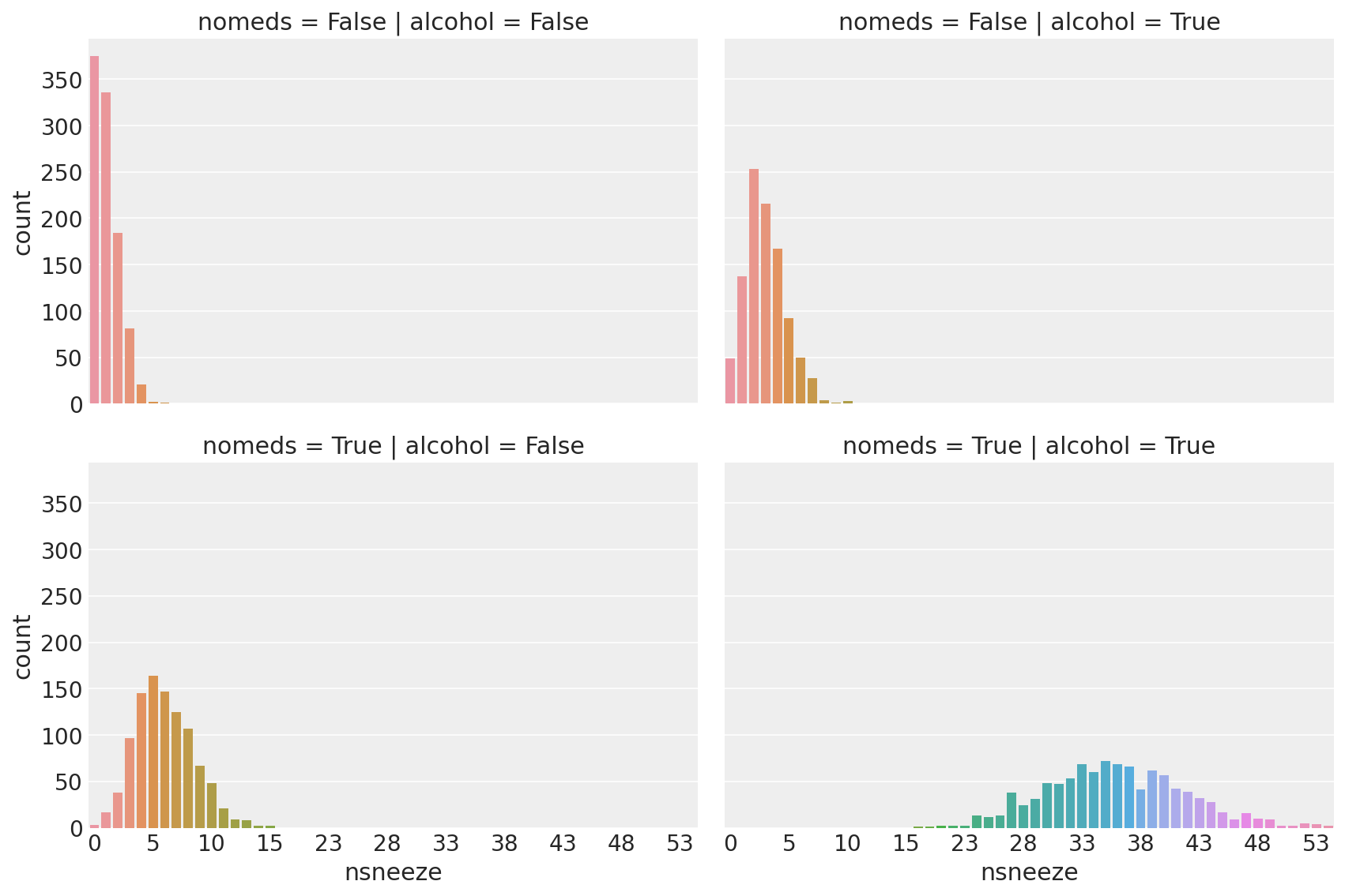
../_images/8d70edc186902abbd997ed8155b0807406213a2113a01aff27e3e638b83321eb.png

Observe:

This looks a lot like poisson-distributed count data (because it is)
With nomeds == False and alcohol == False (top-left, akak antihistamines WERE used, alcohol was NOT drunk) the mean of the poisson distribution of sneeze counts is low.
Changing alcohol == True (top-right) increases the sneeze count nsneeze slightly
Changing nomeds == True (lower-left) increases the sneeze count nsneeze further
Changing both alcohol == True and nomeds == True (lower-right) increases the sneeze count nsneeze a lot, increasing both the mean and variance.

Poisson Regression#

Our model here is a very simple Poisson regression, allowing for interaction of terms:

\[ \theta = exp(\beta X)\]

\[ Y_{sneeze\_count} \sim Poisson(\theta)\]

Create linear model for interaction of terms

fml = "nsneeze ~ alcohol + nomeds + alcohol:nomeds"  # full formulae formulation

fml = "nsneeze ~ alcohol * nomeds"  # lazy, alternative formulae formulation

1. Manual method, create design matrices and manually specify model#

Create Design Matrices

dm = design_matrices(fml, df, na_action="error")

mx_ex = dm.common.as_dataframe()
mx_en = dm.response.as_dataframe()

mx_ex

	Intercept	alcohol	nomeds	alcohol:nomeds
0	1	0	0	0
1	1	0	0	0
2	1	0	0	0
3	1	0	0	0
4	1	0	0	0
...	...	...	...	...
3995	1	1	1	1
3996	1	1	1	1
3997	1	1	1	1
3998	1	1	1	1
3999	1	1	1	1

4000 rows × 4 columns

Create Model

with pm.Model() as mdl_fish:
    # define priors, weakly informative Normal
    b0 = pm.Normal("Intercept", mu=0, sigma=10)
    b1 = pm.Normal("alcohol", mu=0, sigma=10)
    b2 = pm.Normal("nomeds", mu=0, sigma=10)
    b3 = pm.Normal("alcohol:nomeds", mu=0, sigma=10)

    # define linear model and exp link function
    theta = (
        b0
        + b1 * mx_ex["alcohol"].values
        + b2 * mx_ex["nomeds"].values
        + b3 * mx_ex["alcohol:nomeds"].values
    )

    ## Define Poisson likelihood
    y = pm.Poisson("y", mu=pm.math.exp(theta), observed=mx_en["nsneeze"].values)

Sample Model

with mdl_fish:
    inf_fish = pm.sample()
    # inf_fish.extend(pm.sample_posterior_predictive(inf_fish))

Auto-assigning NUTS sampler...
Initializing NUTS using jitter+adapt_diag...
Multiprocess sampling (2 chains in 2 jobs)
NUTS: [Intercept, alcohol, nomeds, alcohol:nomeds]

100.00% [4000/4000 00:24<00:00 Sampling 2 chains, 0 divergences]

Sampling 2 chains for 1_000 tune and 1_000 draw iterations (2_000 + 2_000 draws total) took 36 seconds.

View Diagnostics

az.plot_trace(inf_fish);

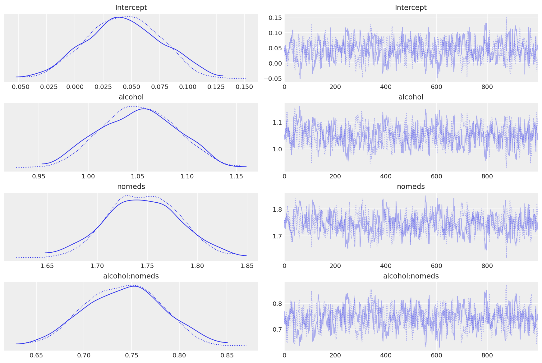
../_images/c2a7d0d9976f8423e0420f0ef0f22992f312119f6def0f7e9a3f6389be9e8e89.png

Observe:

The model converges quickly and traceplots looks pretty well mixed

Transform coeffs and recover theta values#

az.summary(np.exp(inf_fish.posterior), kind="stats")

	mean	sd	hdi_3%	hdi_97%
Intercept	1.045	0.034	0.981	1.106
alcohol	2.862	0.109	2.668	3.065
nomeds	5.734	0.205	5.341	6.115
alcohol:nomeds	2.102	0.086	1.948	2.266

Observe:

The contributions from each feature as a multiplier of the baseline sneezecount appear to be as per the data generation:
1. exp(Intercept): mean=1.05 cr=[0.98, 1.10]
  
  Roughly linear baseline count when no alcohol and meds, as per the generated data:
  
  theta_noalcohol_meds = 1 (as set above) theta_noalcohol_meds = exp(Intercept) = 1
2. exp(alcohol): mean=2.86 cr=[2.67, 3.07]
  
  non-zero positive effect of adding alcohol, a ~3x multiplier of baseline sneeze count, as per the generated data:
  
  theta_alcohol_meds = 3 (as set above) theta_alcohol_meds = exp(Intercept + alcohol) = exp(Intercept) * exp(alcohol) = 1 * 3 = 3
3. exp(nomeds): mean=5.73 cr=[5.34, 6.08]
  
  larger, non-zero positive effect of adding nomeds, a ~6x multiplier of baseline sneeze count, as per the generated data:
  
  theta_noalcohol_nomeds = 6 (as set above) theta_noalcohol_nomeds = exp(Intercept + nomeds) = exp(Intercept) * exp(nomeds) = 1 * 6 = 6
4. exp(alcohol:nomeds): mean=2.10 cr=[1.96, 2.28]
  
  small, positive interaction effect of alcohol and meds, a ~2x multiplier of baseline sneeze count, as per the generated data:
  
  theta_alcohol_nomeds = 36 (as set above) theta_alcohol_nomeds = exp(Intercept + alcohol + nomeds + alcohol:nomeds) = exp(Intercept) * exp(alcohol) * exp(nomeds * alcohol:nomeds) = 1 * 3 * 6 * 2 = 36

2. Alternative method, using `bambi`#

Create Model

Alternative automatic formulation using bambi

model = bmb.Model(fml, df, family="poisson")

Fit Model

inf_fish_alt = model.fit()

Auto-assigning NUTS sampler...
Initializing NUTS using jitter+adapt_diag...
Multiprocess sampling (2 chains in 2 jobs)
NUTS: [Intercept, alcohol, nomeds, alcohol:nomeds]

100.00% [4000/4000 00:27<00:00 Sampling 2 chains, 0 divergences]

Sampling 2 chains for 1_000 tune and 1_000 draw iterations (2_000 + 2_000 draws total) took 36 seconds.

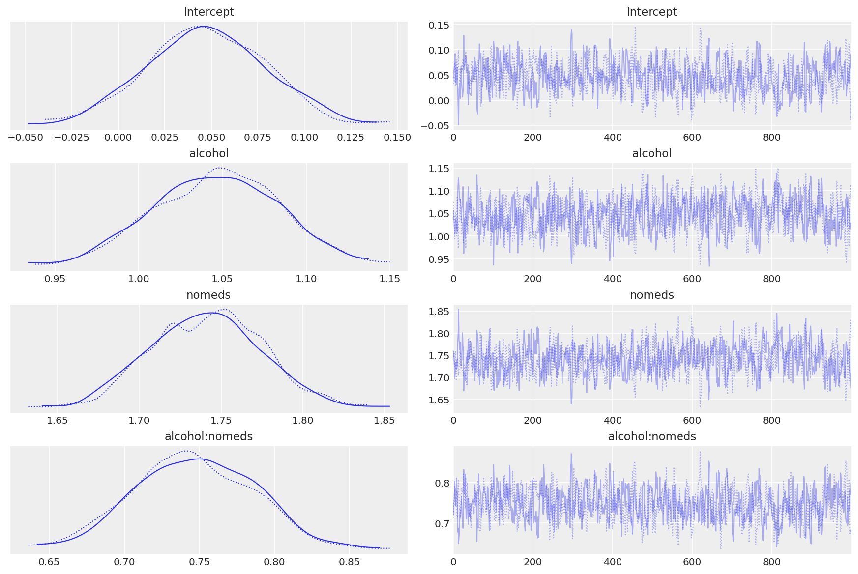
View Traces

az.plot_trace(inf_fish_alt);

../_images/962825f02b34a5cc9b819146b6346d721555ff014a9a51b19018017112debacc.png

Transform coeffs#

az.summary(np.exp(inf_fish_alt.posterior), kind="stats")

	mean	sd	hdi_3%	hdi_97%
Intercept	1.049	0.033	0.987	1.107
alcohol	2.849	0.105	2.659	3.047
nomeds	5.708	0.190	5.362	6.058
alcohol:nomeds	2.111	0.083	1.960	2.258

Observe:

The traceplots look well mixed
The transformed model coeffs look moreorless the same as those generated by the manual model
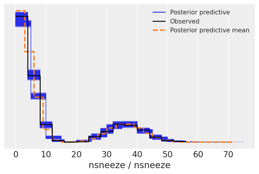
Note that the posterior predictive samples have an extreme skew

posterior_predictive = model.predict(inf_fish_alt, kind="pps")

We can use az.plot_ppc() to check that the posterior predictive samples are similar to the observed data.

For more information on posterior predictive checks, we can refer to Prior and Posterior Predictive Checks.

az.plot_ppc(inf_fish_alt);

../_images/ecad18f81b29b2c6538f64e1933c8cf5c42c93fa3c979e06f6e70dca79b34f4f.png

Authors#

Example originally contributed by Jonathan Sedar 2016-05-15.
Updated to PyMC v4 by Benjamin Vincent May 2022.
Notebook header and footer updated November 2022.

Watermark#

%load_ext watermark
%watermark -n -u -v -iv -w -p pytensor,aeppl

Last updated: Wed Nov 30 2022

Python implementation: CPython
Python version       : 3.10.5
IPython version      : 8.4.0

pytensor: 2.7.5
aeppl : 0.0.32

matplotlib: 3.5.2
seaborn   : 0.12.1
pymc      : 4.1.2
numpy     : 1.21.6
pandas    : 1.4.3
arviz     : 0.12.1
bambi     : 0.9.1

Watermark: 2.3.1

License notice#

All the notebooks in this example gallery are provided under the MIT License which allows modification, and redistribution for any use provided the copyright and license notices are preserved.

Citing PyMC examples#

To cite this notebook, use the DOI provided by Zenodo for the pymc-examples repository.

Important

Many notebooks are adapted from other sources: blogs, books… In such cases you should cite the original source as well.

Also remember to cite the relevant libraries used by your code.

Here is an citation template in bibtex:

@incollection{citekey,
  author    = "<notebook authors, see above>",
  title     = "<notebook title>",
  editor    = "PyMC Team",
  booktitle = "PyMC examples",
  doi       = "10.5281/zenodo.5654871"
}

which once rendered could look like:

Categories

Tags

GLM: Poisson Regression#

Local Functions#

Generate Data#

Assumptions:#

View means of the various combinations (Poisson mean values)#

Briefly Describe Dataset#

Poisson Regression#

1. Manual method, create design matrices and manually specify model#

Transform coeffs and recover theta values#

2. Alternative method, using `bambi`#

Transform coeffs#

Authors#

Watermark#

License notice#

Citing PyMC examples#

Categories

Tags

GLM: Poisson Regression#

Local Functions#

Generate Data#

Assumptions:#

View means of the various combinations (Poisson mean values)#

Briefly Describe Dataset#

Poisson Regression#

1. Manual method, create design matrices and manually specify model#

Transform coeffs and recover theta values#

2. Alternative method, using bambi#

Transform coeffs#

Authors#

Watermark#

License notice#

Citing PyMC examples#

2. Alternative method, using `bambi`#