Discrete Choice and Random Utility Models#
Attention
This notebook uses libraries that are not PyMC dependencies and therefore need to be installed specifically to run this notebook. Open the dropdown below for extra guidance.
Extra dependencies install instructions
In order to run this notebook (either locally or on binder) you won’t only need a working PyMC installation with all optional dependencies, but also to install some extra dependencies. For advise on installing PyMC itself, please refer to Installation
You can install these dependencies with your preferred package manager, we provide as an example the pip and conda commands below.
$ pip install jax, jaxlib, numpyro
Note that if you want (or need) to install the packages from inside the notebook instead of the command line, you can install the packages by running a variation of the pip command:
import sys
!{sys.executable} -m pip install jax, jaxlib, numpyro
You should not run !pip install as it might install the package in a different
environment and not be available from the Jupyter notebook even if installed.
Another alternative is using conda instead:
$ conda install jax, jaxlib, numpyro
when installing scientific python packages with conda, we recommend using conda forge
import arviz as az
import numpy as np  # For vectorized math operations
import pandas as pd  # For file input/output
import pymc as pm
import pytensor.tensor as pt

from matplotlib import pyplot as plt
from matplotlib.lines import Line2D
%config InlineBackend.figure_format = 'retina'  # high resolution figures
az.style.use("arviz-darkgrid")
rng = np.random.default_rng(42)
Discrete Choice Modelling: The Idea#
Discrete choice modelling is related to the idea of a latent utility scale as discussed in Regression Models with Ordered Categorical Outcomes, but it generalises the idea to decision making. It posits that human decision making can be modelled as a function of latent/subjective utility measurements over a set of mutually exclusive alternatives. The theory states that any decision maker will go with the option that maximises their subjective utility, and that utility can be modelled as a latent linear function of observable features of the world.
The idea is perhaps most famously applied by Daniel McFadden in the 1970s to predict the market share accruing to transportation choices (i.e. car, rail, walking etc..) in California after the proposed introduction of BART light rail system. It’s worth pausing on that point. The theory is one of micro level human decision making that has, in real applications, been scaled up to make broadly accurate macro level predictions. For more details we recommend Train [2009]
We don’t need to be too credulous either. This is merely a statistical model and success here is entirely dependent on the skill of modeller and the available measurements coupled with plausible theory. But it’s worth noting the scale of the ambition underlying these models. The structure of the model encourages you to articulate your theory of the decision makers and the environment they inhabit.
The Data#
In this example, we’ll examine the technique of discrete choice modelling using a (i) heating system data set from the R mlogit package and (ii) repeat choice data set over cracker brands. We’ll be pursuing a Bayesian approach to estimating the models rather than the MLE methodology reported in their vigenette. The first data set shows household choices over offers of heating systems in California. The observations consist of single-family houses in California that were newly built and had central air-conditioning. Five types of systems are considered to have been possible:
gas central (gc),
gas room (gr),
electric central (ec),
electric room (er),
heat pump (hp).
The data set reports the installation ic.alt and operating costs oc.alt each household was faced with for each of the five alternatives with some broad demographic information about the household and crucially the choice depvar. This is what one choice scenario over the five alternative looks like in the data:
try:
    wide_heating_df = pd.read_csv("../data/heating_data_r.csv")
except:
    wide_heating_df = pd.read_csv(pm.get_data("heating_data_r.csv"))

wide_heating_df[wide_heating_df["idcase"] == 1]
| idcase | depvar | ic.gc | ic.gr | ic.ec | ic.er | ic.hp | oc.gc | oc.gr | oc.ec | oc.er | oc.hp | income | agehed | rooms | region | |
|---|---|---|---|---|---|---|---|---|---|---|---|---|---|---|---|---|
| 0 | 1 | gc | 866.0 | 962.64 | 859.9 | 995.76 | 1135.5 | 199.69 | 151.72 | 553.34 | 505.6 | 237.88 | 7 | 25 | 6 | ncostl |
The core idea of these kinds of models is to conceive of this scenario as a choice over exhaustive options with attached latent utility. The utility ascribed to each option is viewed as a linear combination of the attributes for each option. The utility ascribed to each alternative drives the probability of choosing amongst each option. For each \(j\) in all the alternatives \(Alt = \{ gc, gr, ec, er, hp \}\) which is assumed to take a Gumbel distribution because this has a particularly nice mathematical property.
This assumption proves to be mathematically convenient because the difference between two Gumbel distributions can be modelled as a logistic function, meaning we can model a contrast difference among multiple alternatives with the softmax function. Details of the derivation can be found in Train [2009]
The model then assumes that decision maker chooses the option that maximises their subjective utility. The individual utility functions can be richly parameterised. The model is identified just when the utility measures of the alternatives are benchmarked against the fixed utility of the “outside good.” The last quantity is fixed at 0.
With all these constraints applied we can build out conditional random utility model and it’s hierarchical variants. Like nearly all subjects in statistics the precise vocabulary for the model specification is overloaded. The conditional logit parameters \(\beta\)
may be fixed at the level of the individual, but can vary across individuals and the alternatives gc, gr, ec, er too. In this manner we can compose an elaborate theory of how we expect drivers of subjective utility to change the market share amongst a set of competing goods.
Digression on Data Formats#
Discrete choice models are often estimated using a long-data format where each choice scenario is represented with a row per alternative ID and a binary flag denoting the chosen option in each scenario. This data format is recommended for estimating these kinds of models in stan and in pylogit. The reason for doing this is that once the columns installation_costs and operating_costs have been pivoted in this fashion it’s easier to include them in matrix calculations.
try:
    long_heating_df = pd.read_csv("../data/long_heating_data.csv")
except:
    long_heating_df = pd.read_csv(pm.get_data("long_heating_data.csv"))

columns = [c for c in long_heating_df.columns if c != "Unnamed: 0"]
long_heating_df[long_heating_df["idcase"] == 1][columns]
| idcase | alt_id | choice | depvar | income | agehed | rooms | region | installation_costs | operating_costs | |
|---|---|---|---|---|---|---|---|---|---|---|
| 0 | 1 | 1 | 1 | gc | 7 | 25 | 6 | ncostl | 866.00 | 199.69 |
| 1 | 1 | 2 | 0 | gc | 7 | 25 | 6 | ncostl | 962.64 | 151.72 |
| 2 | 1 | 3 | 0 | gc | 7 | 25 | 6 | ncostl | 859.90 | 553.34 |
| 3 | 1 | 4 | 0 | gc | 7 | 25 | 6 | ncostl | 995.76 | 505.60 |
| 4 | 1 | 5 | 0 | gc | 7 | 25 | 6 | ncostl | 1135.50 | 237.88 |
The Basic Model#
We will show here how to incorporate the utility specifications in PyMC. PyMC is a nice interface for this kind of modelling because it can express the model quite cleanly following the natural mathematical expression for this system of equations. You can see in this simple model how we go about constructing equations for the utility measure of each alternative seperately, and then stacking them together to create the input matrix for our softmax transform.
N = wide_heating_df.shape[0]
observed = pd.Categorical(wide_heating_df["depvar"]).codes
coords = {
    "alts_probs": ["ec", "er", "gc", "gr", "hp"],
    "obs": range(N),
}

with pm.Model(coords=coords) as model_1:
    beta_ic = pm.Normal("beta_ic", 0, 1)
    beta_oc = pm.Normal("beta_oc", 0, 1)

    ## Construct Utility matrix and Pivot
    u0 = beta_ic * wide_heating_df["ic.ec"] + beta_oc * wide_heating_df["oc.ec"]
    u1 = beta_ic * wide_heating_df["ic.er"] + beta_oc * wide_heating_df["oc.er"]
    u2 = beta_ic * wide_heating_df["ic.gc"] + beta_oc * wide_heating_df["oc.gc"]
    u3 = beta_ic * wide_heating_df["ic.gr"] + beta_oc * wide_heating_df["oc.gr"]
    u4 = np.zeros(N)  # Outside Good
    s = pm.math.stack([u0, u1, u2, u3, u4]).T

    ## Apply Softmax Transform
    p_ = pm.Deterministic("p", pm.math.softmax(s, axis=1), dims=("obs", "alts_probs"))

    ## Likelihood
    choice_obs = pm.Categorical("y_cat", p=p_, observed=observed, dims="obs")

    idata_m1 = pm.sample_prior_predictive()
    idata_m1.extend(
        pm.sample(nuts_sampler="numpyro", idata_kwargs={"log_likelihood": True}, random_seed=101)
    )
    idata_m1.extend(pm.sample_posterior_predictive(idata_m1))

pm.model_to_graphviz(model_1)
Sampling: [beta_ic, beta_oc, y_cat]
/Users/nathanielforde/mambaforge/envs/pymc_examples_new/lib/python3.9/site-packages/pymc/sampling/mcmc.py:243: UserWarning: Use of external NUTS sampler is still experimental
  warnings.warn("Use of external NUTS sampler is still experimental", UserWarning)
Compiling...
Compilation time =  0:00:01.199248
Sampling...
Sampling time =  0:00:02.165671
Transforming variables...
Transformation time =  0:00:00.404064
Computing Log Likelihood...
idata_m1
-
<xarray.Dataset> Dimensions: (chain: 4, draw: 1000, obs: 900, alts_probs: 5) Coordinates: * chain (chain) int64 0 1 2 3 * draw (draw) int64 0 1 2 3 4 5 6 7 ... 992 993 994 995 996 997 998 999 * obs (obs) int64 0 1 2 3 4 5 6 7 ... 892 893 894 895 896 897 898 899 * alts_probs (alts_probs) <U2 'ec' 'er' 'gc' 'gr' 'hp' Data variables: beta_ic (chain, draw) float64 0.001854 0.001794 ... 0.002087 0.001928 beta_oc (chain, draw) float64 -0.003802 -0.003846 ... -0.00447 -0.004533 p (chain, draw, obs, alts_probs) float64 0.07322 0.1129 ... 0.1111 Attributes: created_at: 2023-07-13T17:29:12.988497 arviz_version: 0.15.1 -
<xarray.Dataset> Dimensions: (chain: 4, draw: 1000, obs: 900) Coordinates: * chain (chain) int64 0 1 2 3 * draw (draw) int64 0 1 2 3 4 5 6 7 8 ... 992 993 994 995 996 997 998 999 * obs (obs) int64 0 1 2 3 4 5 6 7 8 ... 892 893 894 895 896 897 898 899 Data variables: y_cat (chain, draw, obs) int64 4 3 4 2 2 1 1 2 4 1 ... 4 3 2 1 4 2 1 1 0 Attributes: created_at: 2023-07-13T17:29:19.656809 arviz_version: 0.15.1 inference_library: pymc inference_library_version: 5.3.0 -
<xarray.Dataset> Dimensions: (chain: 4, draw: 1000, y_cat_dim_0: 1, y_cat_dim_1: 900) Coordinates: * chain (chain) int64 0 1 2 3 * draw (draw) int64 0 1 2 3 4 5 6 7 ... 993 994 995 996 997 998 999 * y_cat_dim_0 (y_cat_dim_0) int64 0 * y_cat_dim_1 (y_cat_dim_1) int64 0 1 2 3 4 5 6 ... 894 895 896 897 898 899 Data variables: y_cat (chain, draw, y_cat_dim_0, y_cat_dim_1) float64 -1.258 ... -... Attributes: created_at: 2023-07-13T17:29:12.992158 arviz_version: 0.15.1 -
<xarray.Dataset> Dimensions: (chain: 4, draw: 1000) Coordinates: * chain (chain) int64 0 1 2 3 * draw (draw) int64 0 1 2 3 4 5 6 ... 993 994 995 996 997 998 999 Data variables: acceptance_rate (chain, draw) float64 0.9667 1.0 0.8868 ... 0.8931 0.9283 step_size (chain, draw) float64 0.02965 0.02965 ... 0.03209 0.03209 diverging (chain, draw) bool False False False ... False False False energy (chain, draw) float64 1.311e+03 1.311e+03 ... 1.312e+03 n_steps (chain, draw) int64 3 3 3 3 1 11 3 7 3 ... 7 7 7 11 7 3 7 3 tree_depth (chain, draw) int64 2 2 2 2 1 4 2 3 2 ... 2 3 3 3 4 3 2 3 2 lp (chain, draw) float64 1.311e+03 1.311e+03 ... 1.311e+03 Attributes: created_at: 2023-07-13T17:29:12.990891 arviz_version: 0.15.1 -
<xarray.Dataset> Dimensions: (chain: 1, draw: 500, obs: 900, alts_probs: 5) Coordinates: * chain (chain) int64 0 * draw (draw) int64 0 1 2 3 4 5 6 7 ... 492 493 494 495 496 497 498 499 * obs (obs) int64 0 1 2 3 4 5 6 7 ... 892 893 894 895 896 897 898 899 * alts_probs (alts_probs) <U2 'ec' 'er' 'gc' 'gr' 'hp' Data variables: beta_oc (chain, draw) float64 0.05221 0.1678 0.7865 ... 0.5232 -0.09242 p (chain, draw, obs, alts_probs) float64 4.778e-201 ... 4.831e-91 beta_ic (chain, draw) float64 -0.57 -0.8283 0.2129 ... 1.097 0.2006 Attributes: created_at: 2023-07-13T17:29:07.842667 arviz_version: 0.15.1 inference_library: pymc inference_library_version: 5.3.0 -
<xarray.Dataset> Dimensions: (chain: 1, draw: 500, obs: 900) Coordinates: * chain (chain) int64 0 * draw (draw) int64 0 1 2 3 4 5 6 7 8 ... 492 493 494 495 496 497 498 499 * obs (obs) int64 0 1 2 3 4 5 6 7 8 ... 892 893 894 895 896 897 898 899 Data variables: y_cat (chain, draw, obs) int64 4 4 4 4 4 4 4 4 4 4 ... 3 1 1 3 3 3 3 3 3 Attributes: created_at: 2023-07-13T17:29:07.844409 arviz_version: 0.15.1 inference_library: pymc inference_library_version: 5.3.0 -
<xarray.Dataset>
Dimensions:  (obs: 900)
Coordinates:
  * obs      (obs) int64 0 1 2 3 4 5 6 7 8 ... 892 893 894 895 896 897 898 899
Data variables:
    y_cat    (obs) int64 2 2 2 1 1 2 2 2 2 2 2 2 2 ... 2 2 2 2 2 2 2 1 2 2 2 2 2
Attributes:
    created_at:                 2023-07-13T17:29:07.844758
    arviz_version:              0.15.1
    inference_library:          pymc
    inference_library_version:  5.3.0
summaries = az.summary(idata_m1, var_names=["beta_ic", "beta_oc"])
summaries
| mean | sd | hdi_3% | hdi_97% | mcse_mean | mcse_sd | ess_bulk | ess_tail | r_hat | |
|---|---|---|---|---|---|---|---|---|---|
| beta_ic | 0.002 | 0.0 | 0.002 | 0.002 | 0.0 | 0.0 | 1870.0 | 1999.0 | 1.0 |
| beta_oc | -0.004 | 0.0 | -0.005 | -0.004 | 0.0 | 0.0 | 881.0 | 1105.0 | 1.0 |
In the mlogit vignette they report how the above model specification leads to inadequate parameter estimates. They note for instance that while the utility scale itself is hard to interpret the value of the ratio of the coefficients is often meaningful because when:
then the marginal rate of substitution is just the ratio of the two beta coefficients. The relative importance of one component of the utility equation to another is an economically meaningful quantity even if the notion of subjective utility is itself unobservable.
Our parameter estimates differ slightly from the reported estimates, but we agree the model is inadequate. We will show a number of Bayesian model checks to demonstrate this fact, but the main call out is that the parameter values for installation costs should probably be negative. It’s counter-intuitive that a \(\beta_{ic}\) increase in price would increase the utility of generated by the installation even marginally as here. Although we might imagine that some kind of quality assurance comes with price which drives satisfaction with higher installation costs. The coefficient for repeat operating costs is negative as expected. Putting this issue aside for now, we’ll show below how we can incorporate prior knowledge to adjust for this kind of conflicts with theory.
But in any case, once we have a fitted model we can calculate the marginal rate of substitution as follows:
## marginal rate of substitution for a reduction in installation costs
post = az.extract(idata_m1)
substitution_rate = post["beta_oc"] / post["beta_ic"]
substitution_rate.mean().item()
-2.215565260325244
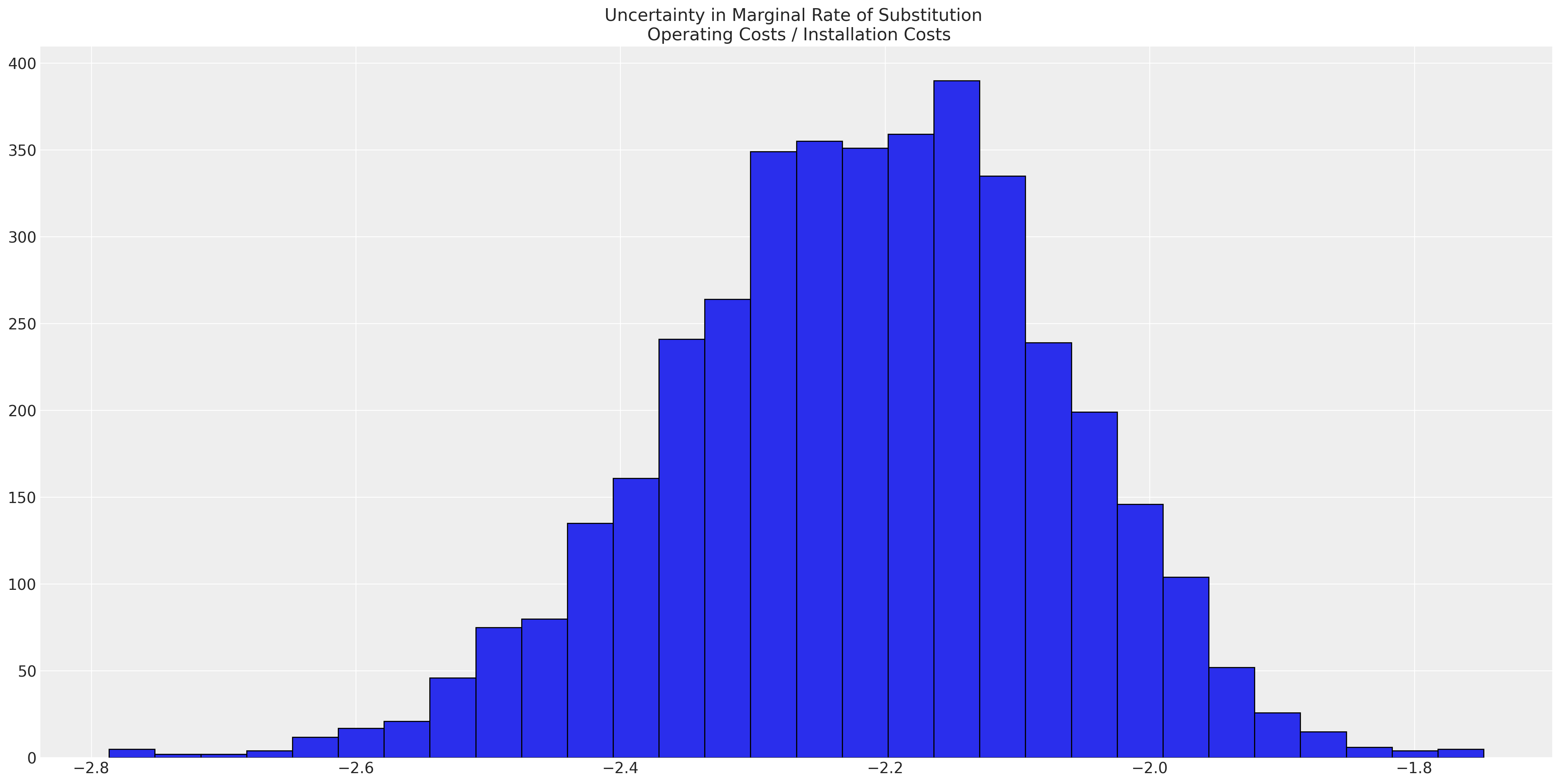
This statistic gives a view of the relative importance of the attributes which drive our utility measures. But being good Bayesians we actually want to calculate the posterior distribution for this statistic.
fig, ax = plt.subplots(figsize=(20, 10))

ax.hist(
    substitution_rate,
    bins=30,
    ec="black",
)
ax.set_title("Uncertainty in Marginal Rate of Substitution \n Operating Costs / Installation Costs");
which suggests that there is almost twice the value accorded to the a unit reduction in recurring operating costs over the one-off installation costs. Whether this is remotely plausible is almost beside the point since the model does not even closely capture the data generating process. But it’s worth repeating that the native scale of utility is not straightforwardly meaningful, but the ratio of the coefficients in the utility equations can be directly interpreted.
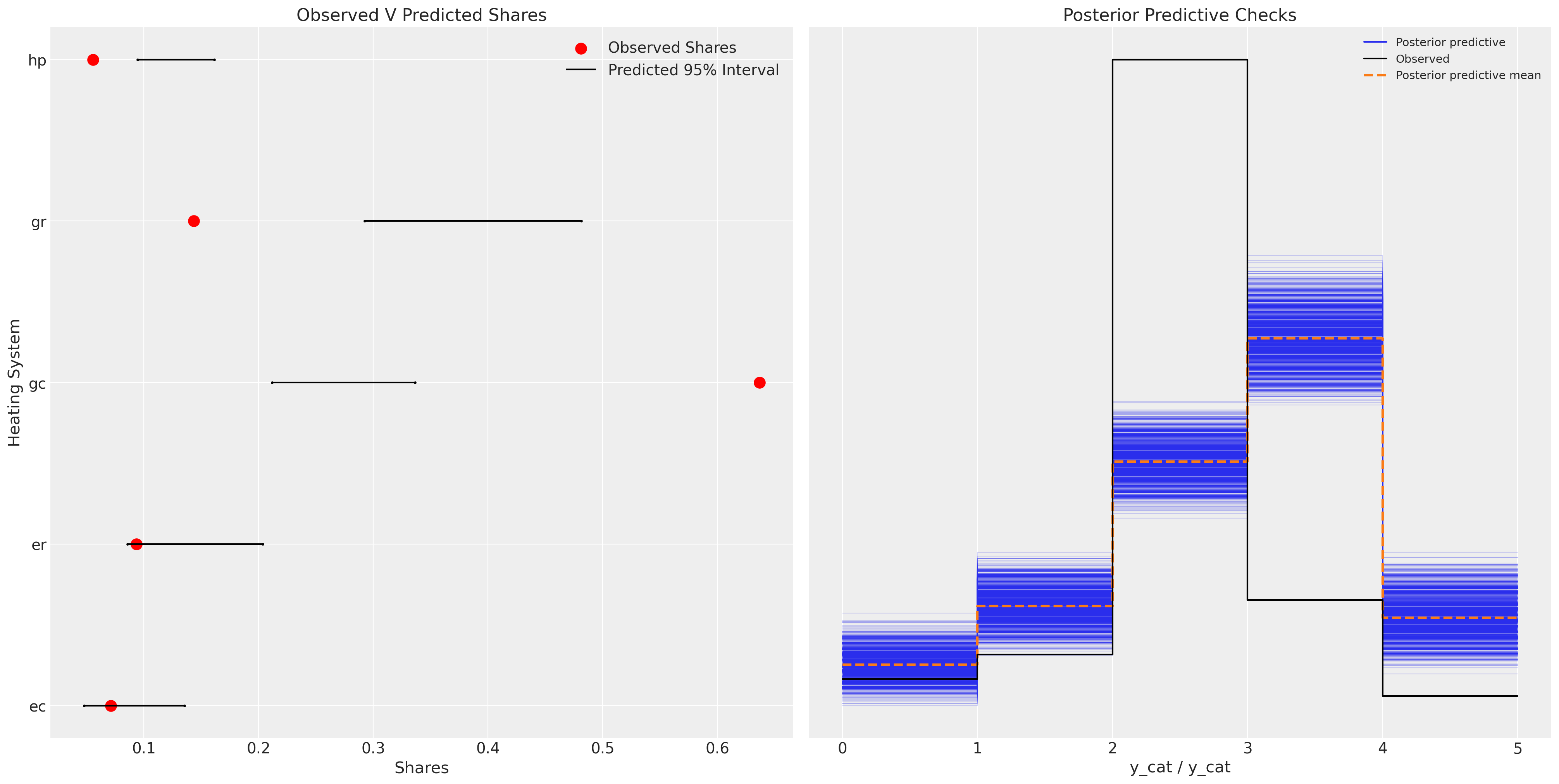
To assess overall model adequacy we can rely on the posterior predictive checks to see if the model can recover an approximation to the data generating process.
idata_m1["posterior"]["p"].mean(dim=["chain", "draw", "obs"])
<xarray.DataArray 'p' (alts_probs: 5)>
array([0.08414602, 0.13748865, 0.26918857, 0.38213088, 0.12704589])
Coordinates:
  * alts_probs  (alts_probs) <U2 'ec' 'er' 'gc' 'gr' 'hp'
fig, axs = plt.subplots(1, 2, figsize=(20, 10))
ax = axs[0]
counts = wide_heating_df.groupby("depvar")["idcase"].count()
predicted_shares = idata_m1["posterior"]["p"].mean(dim=["chain", "draw", "obs"])
ci_lb = idata_m1["posterior"]["p"].quantile(0.025, dim=["chain", "draw", "obs"])
ci_ub = idata_m1["posterior"]["p"].quantile(0.975, dim=["chain", "draw", "obs"])
ax.scatter(ci_lb, ["ec", "er", "gc", "gr", "hp"], color="k", s=2)
ax.scatter(ci_ub, ["ec", "er", "gc", "gr", "hp"], color="k", s=2)
ax.scatter(
    counts / counts.sum(),
    ["ec", "er", "gc", "gr", "hp"],
    label="Observed Shares",
    color="red",
    s=100,
)
ax.hlines(
    ["ec", "er", "gc", "gr", "hp"], ci_lb, ci_ub, label="Predicted 95% Interval", color="black"
)
ax.legend()
ax.set_title("Observed V Predicted Shares")
az.plot_ppc(idata_m1, ax=axs[1])
axs[1].set_title("Posterior Predictive Checks")
ax.set_xlabel("Shares")
ax.set_ylabel("Heating System");
We can see here that the model is fairly inadequate, and fails quite dramatically to recapture the posterior predictive distribution.
Improved Model: Adding Alternative Specific Intercepts#
We can address some of the issues with the prior model specification by adding intercept terms for each of the unique alternatives gr, gc, ec, er. These terms will absorb some of the error seen in the last model by allowing us to control some of the heterogenity of utility measures across products.
N = wide_heating_df.shape[0]
observed = pd.Categorical(wide_heating_df["depvar"]).codes

coords = {
    "alts_intercepts": ["ec", "er", "gc", "gr"],
    "alts_probs": ["ec", "er", "gc", "gr", "hp"],
    "obs": range(N),
}
with pm.Model(coords=coords) as model_2:
    beta_ic = pm.Normal("beta_ic", 0, 1)
    beta_oc = pm.Normal("beta_oc", 0, 1)
    alphas = pm.Normal("alpha", 0, 1, dims="alts_intercepts")

    ## Construct Utility matrix and Pivot using an intercept per alternative
    u0 = alphas[0] + beta_ic * wide_heating_df["ic.ec"] + beta_oc * wide_heating_df["oc.ec"]
    u1 = alphas[1] + beta_ic * wide_heating_df["ic.er"] + beta_oc * wide_heating_df["oc.er"]
    u2 = alphas[2] + beta_ic * wide_heating_df["ic.gc"] + beta_oc * wide_heating_df["oc.gc"]
    u3 = alphas[3] + beta_ic * wide_heating_df["ic.gr"] + beta_oc * wide_heating_df["oc.gr"]
    u4 = np.zeros(N)  # Outside Good
    s = pm.math.stack([u0, u1, u2, u3, u4]).T

    ## Apply Softmax Transform
    p_ = pm.Deterministic("p", pm.math.softmax(s, axis=1), dims=("obs", "alts_probs"))

    ## Likelihood
    choice_obs = pm.Categorical("y_cat", p=p_, observed=observed, dims="obs")

    idata_m2 = pm.sample_prior_predictive()
    idata_m2.extend(
        pm.sample(nuts_sampler="numpyro", idata_kwargs={"log_likelihood": True}, random_seed=103)
    )
    idata_m2.extend(pm.sample_posterior_predictive(idata_m2))


pm.model_to_graphviz(model_2)
Sampling: [alpha, beta_ic, beta_oc, y_cat]
/Users/nathanielforde/mambaforge/envs/pymc_examples_new/lib/python3.9/site-packages/pymc/sampling/mcmc.py:243: UserWarning: Use of external NUTS sampler is still experimental
  warnings.warn("Use of external NUTS sampler is still experimental", UserWarning)
Compiling...
Compilation time =  0:00:01.339706
Sampling...
Sampling time =  0:00:15.309789
Transforming variables...
Transformation time =  0:00:00.289041
Computing Log Likelihood...
az.summary(idata_m2, var_names=["beta_ic", "beta_oc", "alpha"])
| mean | sd | hdi_3% | hdi_97% | mcse_mean | mcse_sd | ess_bulk | ess_tail | r_hat | |
|---|---|---|---|---|---|---|---|---|---|
| beta_ic | 0.001 | 0.000 | -0.000 | 0.001 | 0.000 | 0.000 | 1215.0 | 1612.0 | 1.00 |
| beta_oc | -0.003 | 0.001 | -0.005 | -0.001 | 0.000 | 0.000 | 1379.0 | 1743.0 | 1.00 |
| alpha[ec] | 1.039 | 0.497 | 0.076 | 1.936 | 0.016 | 0.012 | 908.0 | 1054.0 | 1.00 |
| alpha[er] | 1.077 | 0.474 | 0.216 | 1.988 | 0.016 | 0.012 | 839.0 | 991.0 | 1.00 |
| alpha[gc] | 2.376 | 0.309 | 1.789 | 2.953 | 0.011 | 0.008 | 814.0 | 836.0 | 1.01 |
| alpha[gr] | 0.733 | 0.373 | -0.031 | 1.374 | 0.013 | 0.009 | 854.0 | 947.0 | 1.01 |
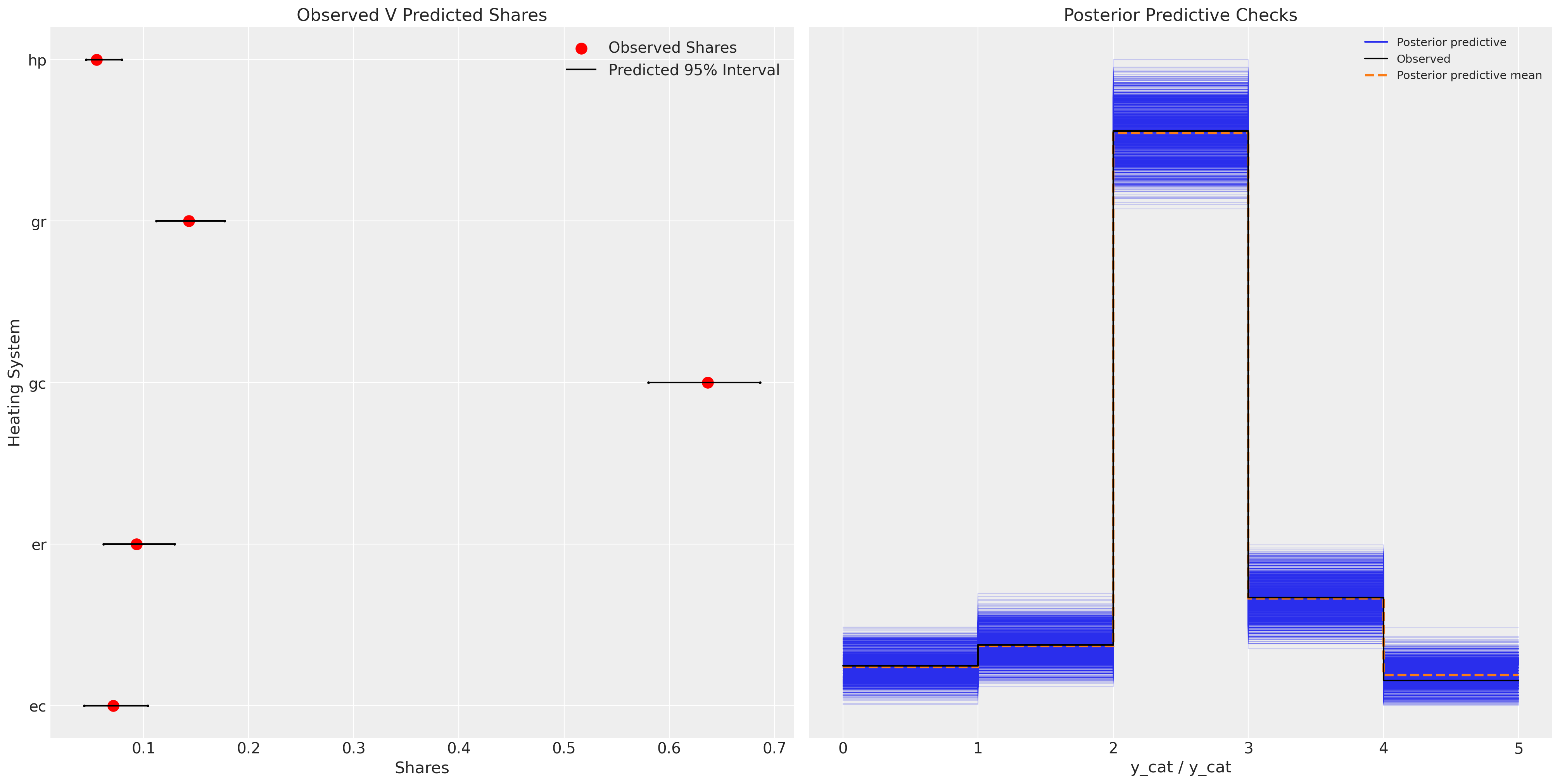
We can see now how this model performs much better in capturing aspects of the data generating process.
fig, axs = plt.subplots(1, 2, figsize=(20, 10))
ax = axs[0]
counts = wide_heating_df.groupby("depvar")["idcase"].count()
predicted_shares = idata_m2["posterior"]["p"].mean(dim=["chain", "draw", "obs"])
ci_lb = idata_m2["posterior"]["p"].quantile(0.025, dim=["chain", "draw", "obs"])
ci_ub = idata_m2["posterior"]["p"].quantile(0.975, dim=["chain", "draw", "obs"])

ax.scatter(ci_lb, ["ec", "er", "gc", "gr", "hp"], color="k", s=2)
ax.scatter(ci_ub, ["ec", "er", "gc", "gr", "hp"], color="k", s=2)
ax.scatter(
    counts / counts.sum(),
    ["ec", "er", "gc", "gr", "hp"],
    label="Observed Shares",
    color="red",
    s=100,
)
ax.hlines(
    ["ec", "er", "gc", "gr", "hp"], ci_lb, ci_ub, label="Predicted 95% Interval", color="black"
)
ax.legend()
ax.set_title("Observed V Predicted Shares")
az.plot_ppc(idata_m2, ax=axs[1])
axs[1].set_title("Posterior Predictive Checks")
ax.set_xlabel("Shares")
ax.set_ylabel("Heating System");
This model represents a substantial improvement.
Experimental Model: Adding Correlation Structure#
We might think that there is a correlation among the alternative goods that we should capture too. We can capture those effects in so far as they exist by placing a multvariate normal prior on the intercepts, (or alternatively the beta parameters). In addition we add information about how the effect of income influences the utility accorded to each alternative.
coords = {
    "alts_intercepts": ["ec", "er", "gc", "gr"],
    "alts_probs": ["ec", "er", "gc", "gr", "hp"],
    "obs": range(N),
}
with pm.Model(coords=coords) as model_3:
    ## Add data to experiment with changes later.
    ic_ec = pm.MutableData("ic_ec", wide_heating_df["ic.ec"])
    oc_ec = pm.MutableData("oc_ec", wide_heating_df["oc.ec"])
    ic_er = pm.MutableData("ic_er", wide_heating_df["ic.er"])
    oc_er = pm.MutableData("oc_er", wide_heating_df["oc.er"])

    beta_ic = pm.Normal("beta_ic", 0, 1)
    beta_oc = pm.Normal("beta_oc", 0, 1)
    beta_income = pm.Normal("beta_income", 0, 1, dims="alts_intercepts")
    chol, corr, stds = pm.LKJCholeskyCov(
        "chol", n=4, eta=2.0, sd_dist=pm.Exponential.dist(1.0, shape=4)
    )
    alphas = pm.MvNormal("alpha", mu=0, chol=chol, dims="alts_intercepts")

    u0 = alphas[0] + beta_ic * ic_ec + beta_oc * oc_ec + beta_income[0] * wide_heating_df["income"]
    u1 = alphas[1] + beta_ic * ic_er + beta_oc * oc_er + beta_income[1] * wide_heating_df["income"]
    u2 = (
        alphas[2]
        + beta_ic * wide_heating_df["ic.gc"]
        + beta_oc * wide_heating_df["oc.gc"]
        + beta_income[2] * wide_heating_df["income"]
    )
    u3 = (
        alphas[3]
        + beta_ic * wide_heating_df["ic.gr"]
        + beta_oc * wide_heating_df["oc.gr"]
        + beta_income[3] * wide_heating_df["income"]
    )
    u4 = np.zeros(N)  # pivot
    s = pm.math.stack([u0, u1, u2, u3, u4]).T

    p_ = pm.Deterministic("p", pm.math.softmax(s, axis=1), dims=("obs", "alts_probs"))
    choice_obs = pm.Categorical("y_cat", p=p_, observed=observed, dims="obs")

    idata_m3 = pm.sample_prior_predictive()
    idata_m3.extend(
        pm.sample(nuts_sampler="numpyro", idata_kwargs={"log_likelihood": True}, random_seed=100)
    )
    idata_m3.extend(pm.sample_posterior_predictive(idata_m3))


pm.model_to_graphviz(model_3)
Sampling: [alpha, beta_ic, beta_income, beta_oc, chol, y_cat]
/Users/nathanielforde/mambaforge/envs/pymc_examples_new/lib/python3.9/site-packages/pymc/sampling/mcmc.py:243: UserWarning: Use of external NUTS sampler is still experimental
  warnings.warn("Use of external NUTS sampler is still experimental", UserWarning)
Compiling...
Compilation time =  0:00:04.533953
Sampling...
Sampling time =  0:00:30.042792
Transforming variables...
Transformation time =  0:00:00.594139
Computing Log Likelihood...
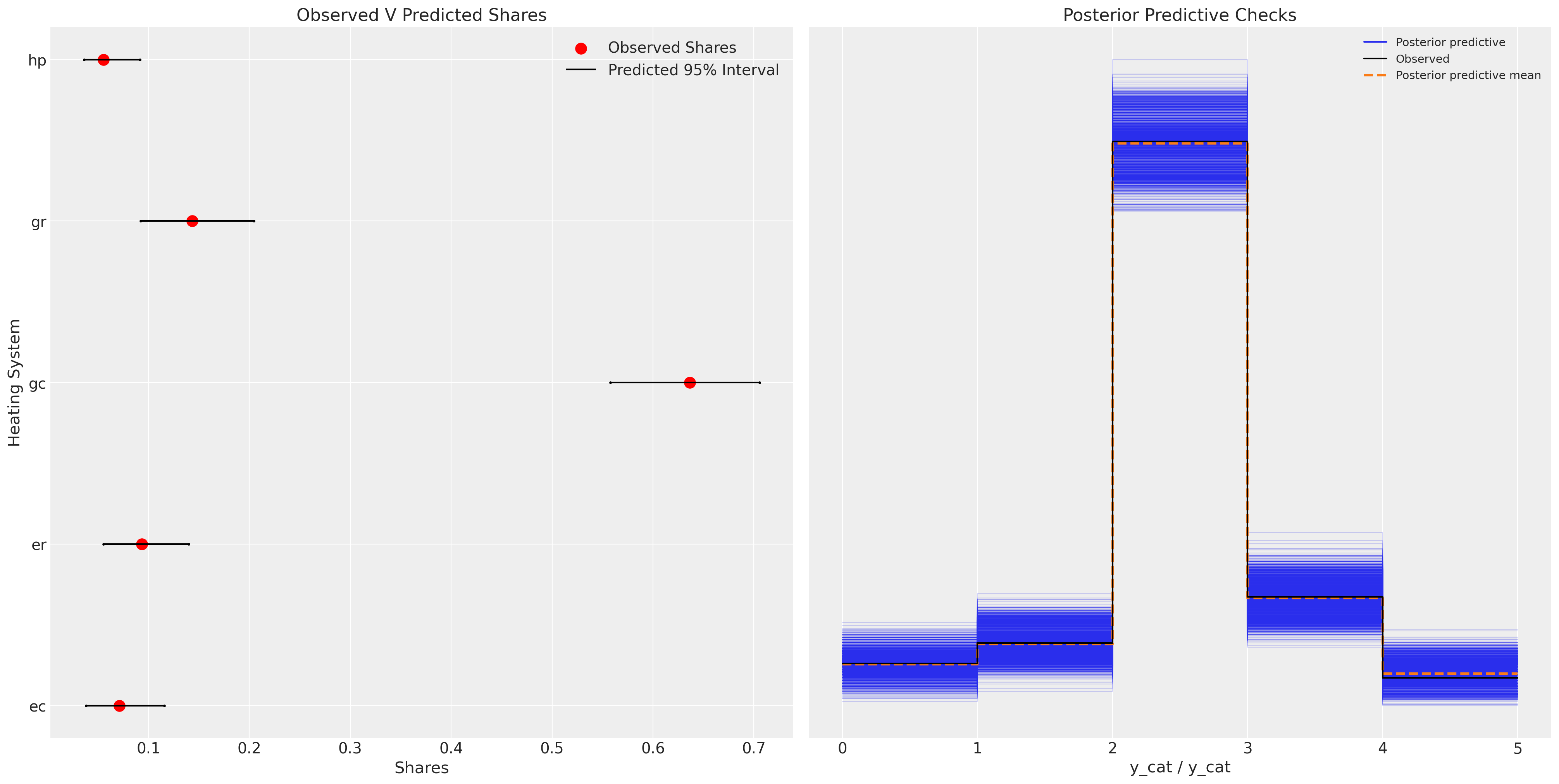
Plotting the model fit we see a similar story.The model predictive performance is not drastically improved and we have added some complexity to the model. This extra complexity ought to be penalised in model assessment metrics such as AIC and WAIC. But often the correlation amongst products are some of the features of interest, independent of issues of historic predictions.
fig, axs = plt.subplots(1, 2, figsize=(20, 10))
ax = axs[0]
counts = wide_heating_df.groupby("depvar")["idcase"].count()
predicted_shares = idata_m3["posterior"]["p"].mean(dim=["chain", "draw", "obs"])
ci_lb = idata_m3["posterior"]["p"].quantile(0.025, dim=["chain", "draw", "obs"])
ci_ub = idata_m3["posterior"]["p"].quantile(0.975, dim=["chain", "draw", "obs"])

ax.scatter(ci_lb, ["ec", "er", "gc", "gr", "hp"], color="k", s=2)
ax.scatter(ci_ub, ["ec", "er", "gc", "gr", "hp"], color="k", s=2)
ax.scatter(
    counts / counts.sum(),
    ["ec", "er", "gc", "gr", "hp"],
    label="Observed Shares",
    color="red",
    s=100,
)
ax.hlines(
    ["ec", "er", "gc", "gr", "hp"], ci_lb, ci_ub, label="Predicted 95% Interval", color="black"
)
ax.legend()
ax.set_title("Observed V Predicted Shares")
az.plot_ppc(idata_m3, ax=axs[1])
axs[1].set_title("Posterior Predictive Checks")
ax.set_xlabel("Shares")
ax.set_ylabel("Heating System");
That extra complexity can be informative, and the degree of relationship amongst the alternative products will inform the substitution patterns under policy changes. Also, note how under this model specification the parameter for beta_ic has a expected value of 0. Suggestive perhaps of a resignation towards the reality of installation costs that doesn’t change the utility metric one way or other after a decision to purchase.
az.summary(
    idata_m3, var_names=["beta_income", "beta_ic", "beta_oc", "alpha", "chol_corr"], round_to=4
)
/Users/nathanielforde/mambaforge/envs/pymc_examples_new/lib/python3.9/site-packages/arviz/stats/diagnostics.py:592: RuntimeWarning: invalid value encountered in double_scalars
  (between_chain_variance / within_chain_variance + num_samples - 1) / (num_samples)
| mean | sd | hdi_3% | hdi_97% | mcse_mean | mcse_sd | ess_bulk | ess_tail | r_hat | |
|---|---|---|---|---|---|---|---|---|---|
| beta_income[ec] | 0.0971 | 0.1074 | -0.1025 | 0.3046 | 0.0035 | 0.0025 | 936.3265 | 1900.0530 | 1.0033 |
| beta_income[er] | 0.0655 | 0.1047 | -0.1187 | 0.2695 | 0.0036 | 0.0025 | 839.1058 | 1613.9147 | 1.0017 |
| beta_income[gc] | 0.0673 | 0.0867 | -0.1058 | 0.2202 | 0.0032 | 0.0023 | 722.9224 | 1321.0255 | 1.0028 |
| beta_income[gr] | -0.0318 | 0.0977 | -0.2220 | 0.1441 | 0.0034 | 0.0024 | 807.8161 | 1624.6096 | 1.0020 |
| beta_ic | 0.0004 | 0.0007 | -0.0009 | 0.0016 | 0.0000 | 0.0000 | 752.9909 | 914.0799 | 1.0019 |
| beta_oc | -0.0035 | 0.0015 | -0.0064 | -0.0007 | 0.0000 | 0.0000 | 1436.0405 | 2066.3187 | 1.0015 |
| alpha[ec] | 1.0354 | 1.0479 | -0.4211 | 3.0541 | 0.0470 | 0.0333 | 520.2449 | 1178.1694 | 1.0063 |
| alpha[er] | 1.2391 | 1.0751 | -0.3175 | 3.2426 | 0.0507 | 0.0358 | 441.6820 | 991.4928 | 1.0064 |
| alpha[gc] | 2.3718 | 0.7613 | 1.1220 | 3.7710 | 0.0366 | 0.0259 | 414.8905 | 699.3486 | 1.0073 |
| alpha[gr] | 1.2014 | 0.8524 | -0.0952 | 2.8006 | 0.0402 | 0.0284 | 442.3913 | 1198.3044 | 1.0053 |
| chol_corr[0, 0] | 1.0000 | 0.0000 | 1.0000 | 1.0000 | 0.0000 | 0.0000 | 4000.0000 | 4000.0000 | NaN |
| chol_corr[0, 1] | 0.1184 | 0.3671 | -0.5402 | 0.7923 | 0.0074 | 0.0062 | 2518.0052 | 2043.9328 | 1.0015 |
| chol_corr[0, 2] | 0.1427 | 0.3705 | -0.5480 | 0.7769 | 0.0093 | 0.0066 | 1673.7845 | 1975.7307 | 1.0020 |
| chol_corr[0, 3] | 0.1157 | 0.3753 | -0.5676 | 0.7683 | 0.0079 | 0.0056 | 2319.4753 | 2119.7780 | 1.0012 |
| chol_corr[1, 0] | 0.1184 | 0.3671 | -0.5402 | 0.7923 | 0.0074 | 0.0062 | 2518.0052 | 2043.9328 | 1.0015 |
| chol_corr[1, 1] | 1.0000 | 0.0000 | 1.0000 | 1.0000 | 0.0000 | 0.0000 | 4239.6296 | 4000.0000 | 0.9996 |
| chol_corr[1, 2] | 0.1675 | 0.3483 | -0.4430 | 0.8095 | 0.0079 | 0.0056 | 1978.9399 | 1538.2851 | 1.0011 |
| chol_corr[1, 3] | 0.1526 | 0.3561 | -0.4722 | 0.7963 | 0.0070 | 0.0050 | 2595.1991 | 3126.5524 | 1.0014 |
| chol_corr[2, 0] | 0.1427 | 0.3705 | -0.5480 | 0.7769 | 0.0093 | 0.0066 | 1673.7845 | 1975.7307 | 1.0020 |
| chol_corr[2, 1] | 0.1675 | 0.3483 | -0.4430 | 0.8095 | 0.0079 | 0.0056 | 1978.9399 | 1538.2851 | 1.0011 |
| chol_corr[2, 2] | 1.0000 | 0.0000 | 1.0000 | 1.0000 | 0.0000 | 0.0000 | 3929.0431 | 4000.0000 | 1.0007 |
| chol_corr[2, 3] | 0.1757 | 0.3411 | -0.4384 | 0.7867 | 0.0071 | 0.0051 | 2260.6724 | 2564.2728 | 1.0017 |
| chol_corr[3, 0] | 0.1157 | 0.3753 | -0.5676 | 0.7683 | 0.0079 | 0.0056 | 2319.4753 | 2119.7780 | 1.0012 |
| chol_corr[3, 1] | 0.1526 | 0.3561 | -0.4722 | 0.7963 | 0.0070 | 0.0050 | 2595.1991 | 3126.5524 | 1.0014 |
| chol_corr[3, 2] | 0.1757 | 0.3411 | -0.4384 | 0.7867 | 0.0071 | 0.0051 | 2260.6724 | 2564.2728 | 1.0017 |
| chol_corr[3, 3] | 1.0000 | 0.0000 | 1.0000 | 1.0000 | 0.0000 | 0.0000 | 3954.4789 | 3702.0363 | 1.0001 |
In this model we see that the marginal rate of substitution shows that an increase of one dollar for the operating costs is almost 17 times more impactful on the utility calculus than a similar increase in installation costs. Which makes sense in so far as we can expect the installation costs to be a one-off expense we’re pretty resigned to.
post = az.extract(idata_m3)
substitution_rate = post["beta_oc"] / post["beta_ic"]
substitution_rate.mean().item()
17.581376035151784
Compare Models#
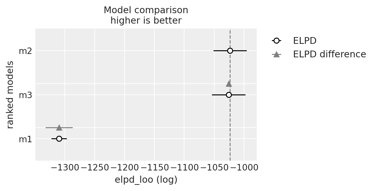
We’ll now evaluate all three model fits on their predictive performance. Predictive performance on the original data is a good benchmark that the model has appropriately captured the data generating process. But it is not (as we’ve seen) the only feature of interest in these models. These models are sensetive to our theoretical beliefs about the agents making the decisions, the view of the decision process and the elements of the choice scenario.
compare = az.compare({"m1": idata_m1, "m2": idata_m2, "m3": idata_m3})
compare
| rank | elpd_loo | p_loo | elpd_diff | weight | se | dse | warning | scale | |
|---|---|---|---|---|---|---|---|---|---|
| m2 | 0 | -1023.600927 | 4.964862 | 0.000000 | 1.000000e+00 | 27.802379 | 0.000000 | False | log |
| m3 | 1 | -1025.830780 | 9.954792 | 2.229854 | 2.220446e-16 | 28.086804 | 2.070976 | False | log |
| m1 | 2 | -1309.610895 | 1.196878 | 286.009968 | 0.000000e+00 | 12.933024 | 22.677606 | False | log |
az.plot_compare(compare)
Choosing Crackers over Repeated Choices: Mixed Logit Model#
Moving to another example, we see a choice scenario where the same individual has been repeatedly polled on their choice of crackers among alternatives. This affords us the opportunity to evaluate the preferences of individuals by adding in coefficients for individuals for each product.
try:
    c_df = pd.read_csv("../data/cracker_choice_short.csv")
except:
    c_df = pd.read_csv(pm.get_data("cracker_choice_short.csv"))
columns = [c for c in c_df.columns if c != "Unnamed: 0"]
c_df[columns]
| personId | disp.sunshine | disp.keebler | disp.nabisco | disp.private | feat.sunshine | feat.keebler | feat.nabisco | feat.private | price.sunshine | price.keebler | price.nabisco | price.private | choice | lastChoice | personChoiceId | choiceId | |
|---|---|---|---|---|---|---|---|---|---|---|---|---|---|---|---|---|---|
| 0 | 1 | 0 | 0 | 0 | 0 | 0 | 0 | 0 | 0 | 0.99 | 1.09 | 0.99 | 0.71 | nabisco | nabisco | 1 | 1 |
| 1 | 1 | 1 | 0 | 0 | 0 | 0 | 0 | 0 | 0 | 0.49 | 1.09 | 1.09 | 0.78 | sunshine | nabisco | 2 | 2 |
| 2 | 1 | 0 | 0 | 0 | 0 | 0 | 0 | 0 | 0 | 1.03 | 1.09 | 0.89 | 0.78 | nabisco | sunshine | 3 | 3 |
| 3 | 1 | 0 | 0 | 0 | 0 | 0 | 0 | 0 | 0 | 1.09 | 1.09 | 1.19 | 0.64 | nabisco | nabisco | 4 | 4 |
| 4 | 1 | 0 | 0 | 0 | 0 | 0 | 0 | 0 | 0 | 0.89 | 1.09 | 1.19 | 0.84 | nabisco | nabisco | 5 | 5 |
| ... | ... | ... | ... | ... | ... | ... | ... | ... | ... | ... | ... | ... | ... | ... | ... | ... | ... |
| 3151 | 136 | 0 | 0 | 0 | 0 | 0 | 0 | 0 | 0 | 1.09 | 1.19 | 0.99 | 0.55 | private | private | 9 | 3152 |
| 3152 | 136 | 0 | 0 | 0 | 1 | 0 | 0 | 0 | 0 | 0.78 | 1.35 | 1.04 | 0.65 | private | private | 10 | 3153 |
| 3153 | 136 | 0 | 0 | 0 | 0 | 0 | 0 | 0 | 0 | 1.09 | 1.17 | 1.29 | 0.59 | private | private | 11 | 3154 |
| 3154 | 136 | 0 | 0 | 0 | 0 | 0 | 0 | 0 | 0 | 1.09 | 1.22 | 1.29 | 0.59 | private | private | 12 | 3155 |
| 3155 | 136 | 0 | 0 | 0 | 0 | 0 | 0 | 0 | 0 | 1.29 | 1.04 | 1.23 | 0.59 | private | private | 13 | 3156 |
3156 rows × 17 columns
c_df.groupby("personId")[["choiceId"]].count().T
| personId | 1 | 2 | 3 | 4 | 5 | 6 | 7 | 8 | 9 | 10 | ... | 127 | 128 | 129 | 130 | 131 | 132 | 133 | 134 | 135 | 136 |
|---|---|---|---|---|---|---|---|---|---|---|---|---|---|---|---|---|---|---|---|---|---|
| choiceId | 15 | 15 | 13 | 28 | 13 | 27 | 16 | 25 | 18 | 40 | ... | 17 | 25 | 31 | 31 | 29 | 21 | 26 | 13 | 14 | 13 |
1 rows × 136 columns
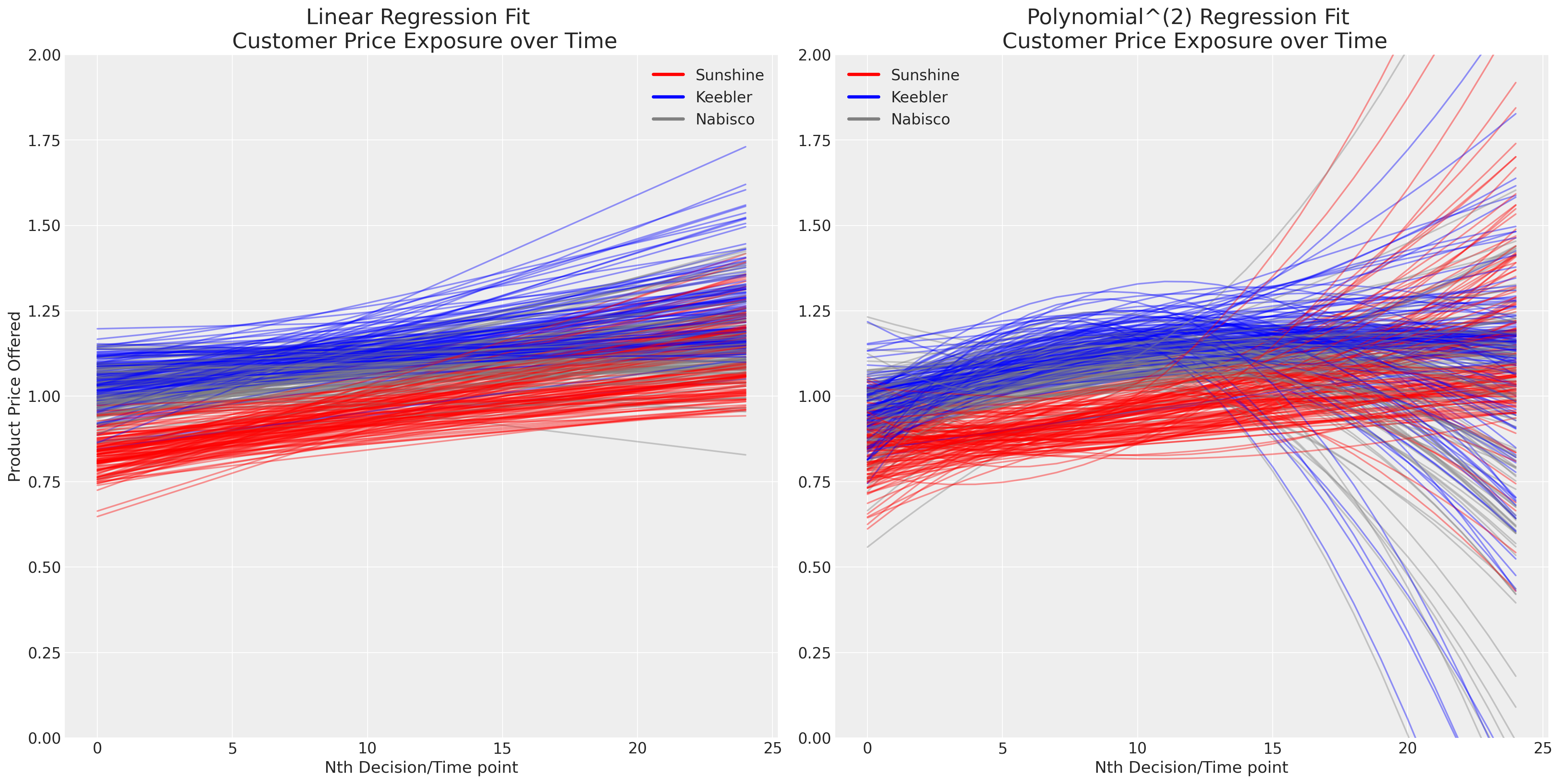
The presence of repeated choice over time complicates the issue. We now have to contend with issues of personal taste and the evolving or dynamic effects of pricing in a competitive environment. Plotting the simple linear and polynomial fits for each person’s successive exposure to the brand price, seems to suggest that (a) pricing differentiates the product offering and (b) pricing evolves over time.
fig, axs = plt.subplots(1, 2, figsize=(20, 10))
axs = axs.flatten()
map_color = {"nabisco": "red", "keebler": "blue", "sunshine": "purple", "private": "orange"}


for i in c_df["personId"].unique():
    temp = c_df[c_df["personId"] == i].copy(deep=True)
    temp["color"] = temp["choice"].map(map_color)
    predict = np.poly1d(np.polyfit(temp["personChoiceId"], temp["price.sunshine"], deg=1))
    axs[0].plot(predict(range(25)), color="red", label="Sunshine", alpha=0.4)
    predict = np.poly1d(np.polyfit(temp["personChoiceId"], temp["price.keebler"], deg=1))
    axs[0].plot(predict(range(25)), color="blue", label="Keebler", alpha=0.4)
    predict = np.poly1d(np.polyfit(temp["personChoiceId"], temp["price.nabisco"], deg=1))
    axs[0].plot(predict(range(25)), color="grey", label="Nabisco", alpha=0.4)

    predict = np.poly1d(np.polyfit(temp["personChoiceId"], temp["price.sunshine"], deg=2))
    axs[1].plot(predict(range(25)), color="red", label="Sunshine", alpha=0.4)
    predict = np.poly1d(np.polyfit(temp["personChoiceId"], temp["price.keebler"], deg=2))
    axs[1].plot(predict(range(25)), color="blue", label="Keebler", alpha=0.4)
    predict = np.poly1d(np.polyfit(temp["personChoiceId"], temp["price.nabisco"], deg=2))
    axs[1].plot(predict(range(25)), color="grey", label="Nabisco", alpha=0.4)

axs[0].set_title("Linear Regression Fit \n Customer Price Exposure over Time", fontsize=20)
axs[1].set_title("Polynomial^(2) Regression Fit \n Customer Price Exposure over Time", fontsize=20)
axs[0].set_xlabel("Nth Decision/Time point")
axs[1].set_xlabel("Nth Decision/Time point")
axs[0].set_ylabel("Product Price Offered")
axs[1].set_ylim(0, 2)
axs[0].set_ylim(0, 2)

colors = ["red", "blue", "grey"]
lines = [Line2D([0], [0], color=c, linewidth=3, linestyle="-") for c in colors]
labels = ["Sunshine", "Keebler", "Nabisco"]
axs[0].legend(lines, labels)
axs[1].legend(lines, labels);
We’ll model now how individual taste enters into discrete choice problems, but ignore the complexities of the time-dimension or the endogenity of price in the system. There are adaptions of the basic discrete choice model that are designed to address each of these complications. We’ll leave the temporal dynamics as a suggested exercise for the reader.
N = c_df.shape[0]
observed = pd.Categorical(c_df["choice"]).codes
person_indx, uniques = pd.factorize(c_df["personId"])

coords = {
    "alts_intercepts": ["sunshine", "keebler", "nabisco"],
    "alts_probs": ["sunshine", "keebler", "nabisco", "private"],
    "individuals": uniques,
    "obs": range(N),
}
with pm.Model(coords=coords) as model_4:
    beta_feat = pm.TruncatedNormal("beta_feat", 0, 1, upper=10, lower=0)
    beta_disp = pm.TruncatedNormal("beta_disp", 0, 1, upper=10, lower=0)
    ## Stronger Prior on Price to ensure an increase in price negatively impacts utility
    beta_price = pm.TruncatedNormal("beta_price", 0, 1, upper=0, lower=-10)
    alphas = pm.Normal("alpha", 0, 1, dims="alts_intercepts")
    beta_individual = pm.Normal("beta_individual", 0, 0.05, dims=("individuals", "alts_intercepts"))

    u0 = (
        (alphas[0] + beta_individual[person_indx, 0])
        + beta_disp * c_df["disp.sunshine"]
        + beta_feat * c_df["feat.sunshine"]
        + beta_price * c_df["price.sunshine"]
    )
    u1 = (
        (alphas[1] + beta_individual[person_indx, 1])
        + beta_disp * c_df["disp.keebler"]
        + beta_feat * c_df["feat.keebler"]
        + beta_price * c_df["price.keebler"]
    )
    u2 = (
        (alphas[2] + beta_individual[person_indx, 2])
        + beta_disp * c_df["disp.nabisco"]
        + beta_feat * c_df["feat.nabisco"]
        + beta_price * c_df["price.nabisco"]
    )
    u3 = np.zeros(N)  # Outside Good
    s = pm.math.stack([u0, u1, u2, u3]).T
    # Reconstruct the total data

    ## Apply Softmax Transform
    p_ = pm.Deterministic("p", pm.math.softmax(s, axis=1), dims=("obs", "alts_probs"))

    ## Likelihood
    choice_obs = pm.Categorical("y_cat", p=p_, observed=observed, dims="obs")

    idata_m4 = pm.sample_prior_predictive()
    idata_m4.extend(
        pm.sample(nuts_sampler="numpyro", idata_kwargs={"log_likelihood": True}, random_seed=103)
    )
    idata_m4.extend(pm.sample_posterior_predictive(idata_m4))


pm.model_to_graphviz(model_4)
Sampling: [alpha, beta_disp, beta_feat, beta_individual, beta_price, y_cat]
/Users/nathanielforde/mambaforge/envs/pymc_examples_new/lib/python3.9/site-packages/pymc/sampling/mcmc.py:243: UserWarning: Use of external NUTS sampler is still experimental
  warnings.warn("Use of external NUTS sampler is still experimental", UserWarning)
Compiling...
Compilation time =  0:00:02.628050
Sampling...
Sampling time =  0:00:11.040460
Transforming variables...
Transformation time =  0:00:01.419801
Computing Log Likelihood...
az.summary(idata_m4, var_names=["beta_disp", "beta_feat", "beta_price", "alpha", "beta_individual"])
| mean | sd | hdi_3% | hdi_97% | mcse_mean | mcse_sd | ess_bulk | ess_tail | r_hat | |
|---|---|---|---|---|---|---|---|---|---|
| beta_disp | 0.023 | 0.021 | 0.000 | 0.061 | 0.000 | 0.000 | 5386.0 | 2248.0 | 1.0 |
| beta_feat | 0.019 | 0.018 | 0.000 | 0.052 | 0.000 | 0.000 | 6417.0 | 2283.0 | 1.0 |
| beta_price | -0.021 | 0.020 | -0.059 | -0.000 | 0.000 | 0.000 | 4281.0 | 2277.0 | 1.0 |
| alpha[sunshine] | -0.054 | 0.096 | -0.243 | 0.119 | 0.002 | 0.001 | 3632.0 | 3220.0 | 1.0 |
| alpha[keebler] | 2.023 | 0.073 | 1.886 | 2.159 | 0.001 | 0.001 | 3302.0 | 2894.0 | 1.0 |
| ... | ... | ... | ... | ... | ... | ... | ... | ... | ... |
| beta_individual[135, keebler] | 0.012 | 0.048 | -0.077 | 0.104 | 0.000 | 0.001 | 10419.0 | 3135.0 | 1.0 |
| beta_individual[135, nabisco] | -0.009 | 0.051 | -0.108 | 0.081 | 0.000 | 0.001 | 10504.0 | 2555.0 | 1.0 |
| beta_individual[136, sunshine] | -0.002 | 0.049 | -0.089 | 0.096 | 0.001 | 0.001 | 7867.0 | 2729.0 | 1.0 |
| beta_individual[136, keebler] | -0.018 | 0.048 | -0.112 | 0.071 | 0.001 | 0.001 | 7684.0 | 2845.0 | 1.0 |
| beta_individual[136, nabisco] | 0.020 | 0.050 | -0.072 | 0.114 | 0.001 | 0.001 | 8252.0 | 2559.0 | 1.0 |
414 rows × 9 columns
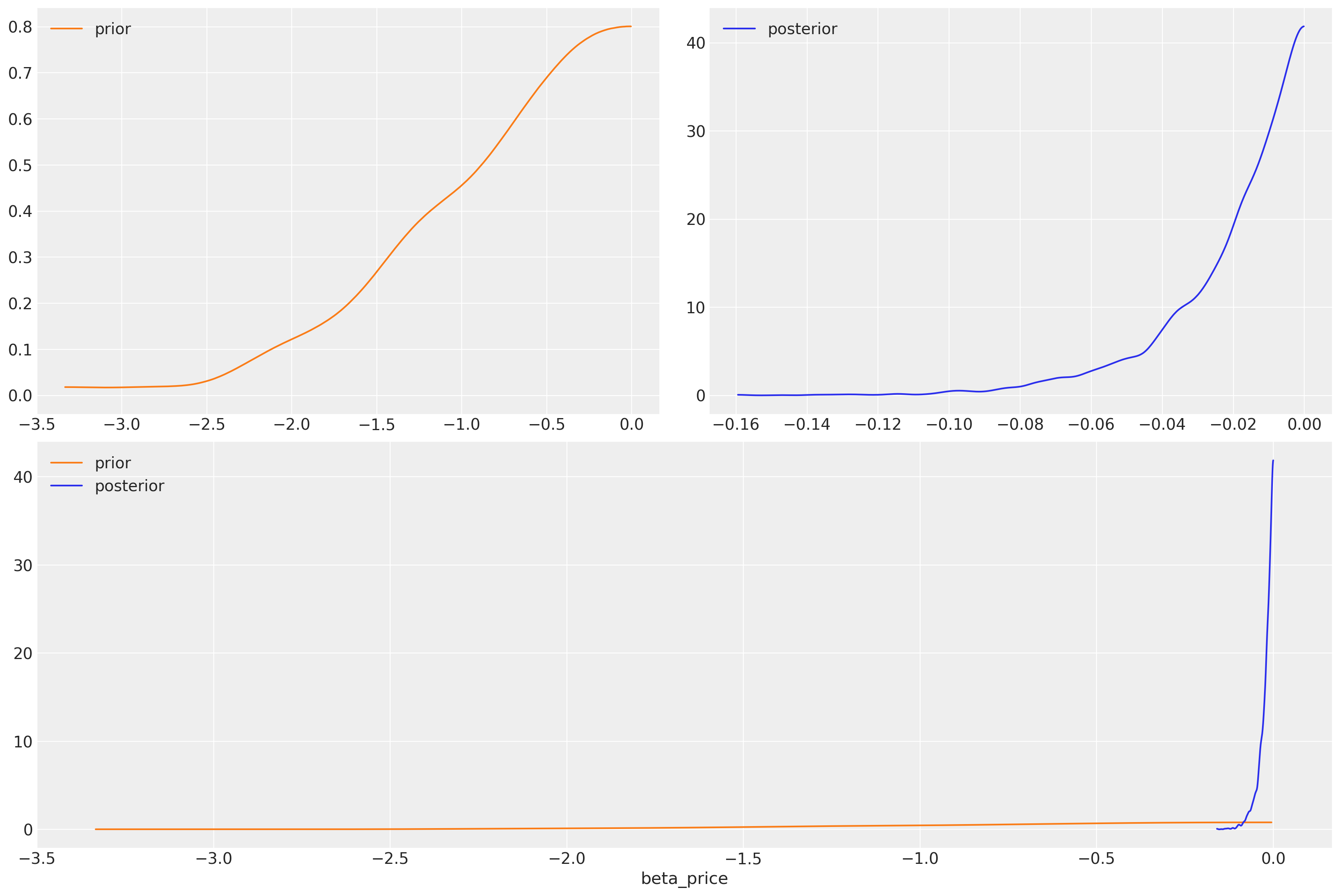
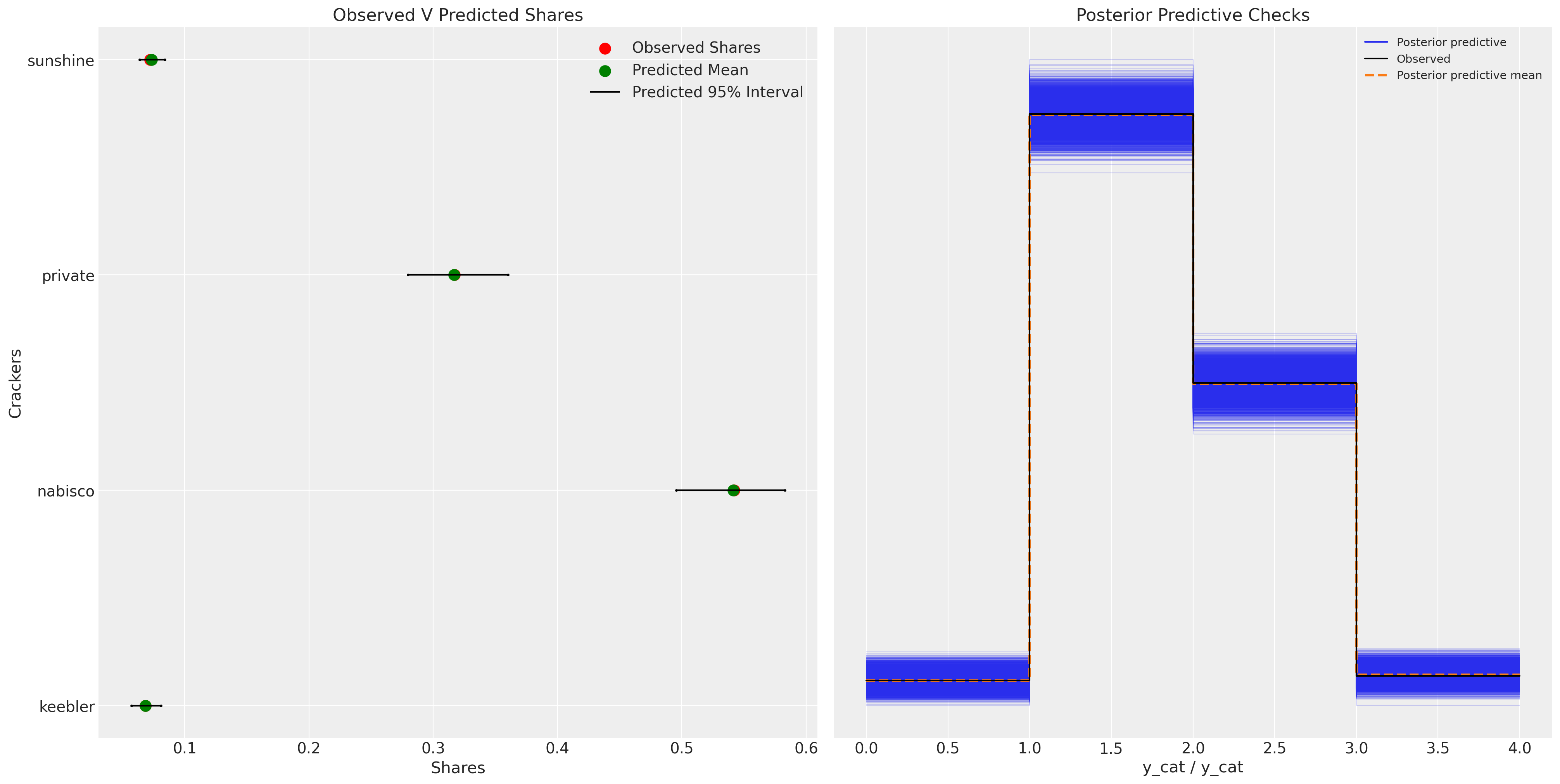
What have we learned? We’ve imposed a negative slope on the price coefficient but given it a wide prior. We can see that the data is sufficient to have narrowed the likely range of the coefficient considerably.
az.plot_dist_comparison(idata_m4, var_names=["beta_price"]);
We have explicitly set a negative prior on price and recovered a parameter specification more in line with the basic theory of rational choice. The effect of price should have a negative impact on utility. The flexibility of priors here is key for incorporating theoretical knowledge about the process involved in choice. Priors are important for building a better picture of the decision making process and we’d be foolish to ignore their value in this setting.
fig, axs = plt.subplots(1, 2, figsize=(20, 10))
ax = axs[0]
counts = c_df.groupby("choice")["choiceId"].count()
labels = c_df.groupby("choice")["choiceId"].count().index
predicted_shares = idata_m4["posterior"]["p"].mean(dim=["chain", "draw", "obs"])
ci_lb = idata_m4["posterior"]["p"].quantile(0.025, dim=["chain", "draw", "obs"])
ci_ub = idata_m4["posterior"]["p"].quantile(0.975, dim=["chain", "draw", "obs"])
ax.scatter(ci_lb, labels, color="k", s=2)
ax.scatter(ci_ub, labels, color="k", s=2)
ax.scatter(
    counts / counts.sum(),
    labels,
    label="Observed Shares",
    color="red",
    s=100,
)
ax.scatter(
    predicted_shares,
    labels,
    label="Predicted Mean",
    color="green",
    s=100,
)
ax.hlines(
    labels,
    ci_lb,
    ci_ub,
    label="Predicted 95% Interval",
    color="black",
)
ax.legend()
ax.set_title("Observed V Predicted Shares")
az.plot_ppc(idata_m4, ax=axs[1])
axs[1].set_title("Posterior Predictive Checks")
ax.set_xlabel("Shares")
ax.set_ylabel("Crackers");
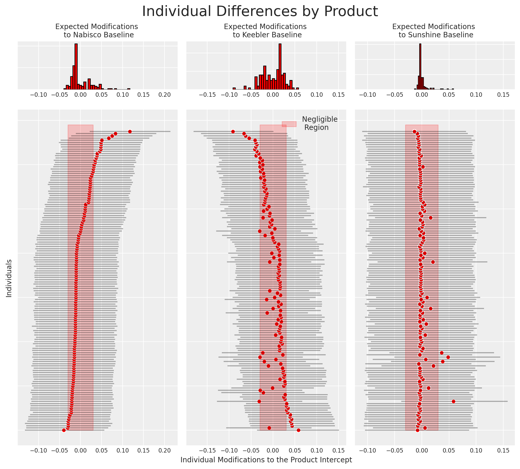
We can now also recover the differences among individuals estimated by the model for particular cracker choices. More precisely we’ll plot how the individual specific contribution to the intercept drives preferences among the cracker choices.
idata_m4
-
<xarray.Dataset> Dimensions: (chain: 4, draw: 1000, alts_intercepts: 3, individuals: 136, obs: 3156, alts_probs: 4) Coordinates: * chain (chain) int64 0 1 2 3 * draw (draw) int64 0 1 2 3 4 5 6 ... 993 994 995 996 997 998 999 * alts_intercepts (alts_intercepts) <U8 'sunshine' 'keebler' 'nabisco' * individuals (individuals) int64 1 2 3 4 5 6 ... 131 132 133 134 135 136 * obs (obs) int64 0 1 2 3 4 5 6 ... 3150 3151 3152 3153 3154 3155 * alts_probs (alts_probs) <U8 'sunshine' 'keebler' 'nabisco' 'private' Data variables: alpha (chain, draw, alts_intercepts) float64 -0.03604 ... 1.472 beta_individual (chain, draw, individuals, alts_intercepts) float64 -0.0... beta_feat (chain, draw) float64 0.008284 0.00381 ... 0.06727 0.0183 beta_disp (chain, draw) float64 0.02731 0.02334 ... 0.003561 0.001434 beta_price (chain, draw) float64 -0.01967 -0.08042 ... -0.01557 p (chain, draw, obs, alts_probs) float64 0.05909 ... 0.07105 Attributes: created_at: 2023-07-13T17:31:22.499390 arviz_version: 0.15.1 -
<xarray.Dataset> Dimensions: (chain: 4, draw: 1000, obs: 3156) Coordinates: * chain (chain) int64 0 1 2 3 * draw (draw) int64 0 1 2 3 4 5 6 7 8 ... 992 993 994 995 996 997 998 999 * obs (obs) int64 0 1 2 3 4 5 6 7 ... 3149 3150 3151 3152 3153 3154 3155 Data variables: y_cat (chain, draw, obs) int64 2 0 1 2 2 1 2 2 1 1 ... 2 1 2 2 1 1 2 2 1 Attributes: created_at: 2023-07-13T17:31:45.522950 arviz_version: 0.15.1 inference_library: pymc inference_library_version: 5.3.0 -
<xarray.Dataset> Dimensions: (chain: 4, draw: 1000, y_cat_dim_0: 1, y_cat_dim_1: 3156) Coordinates: * chain (chain) int64 0 1 2 3 * draw (draw) int64 0 1 2 3 4 5 6 7 ... 993 994 995 996 997 998 999 * y_cat_dim_0 (y_cat_dim_0) int64 0 * y_cat_dim_1 (y_cat_dim_1) int64 0 1 2 3 4 5 ... 3151 3152 3153 3154 3155 Data variables: y_cat (chain, draw, y_cat_dim_0, y_cat_dim_1) float64 -0.5664 ... ... Attributes: created_at: 2023-07-13T17:31:22.503457 arviz_version: 0.15.1 -
<xarray.Dataset> Dimensions: (chain: 4, draw: 1000) Coordinates: * chain (chain) int64 0 1 2 3 * draw (draw) int64 0 1 2 3 4 5 6 ... 993 994 995 996 997 998 999 Data variables: acceptance_rate (chain, draw) float64 0.7536 1.0 0.832 ... 0.5635 0.7482 step_size (chain, draw) float64 0.3084 0.3084 ... 0.3254 0.3254 diverging (chain, draw) bool False False False ... False False False energy (chain, draw) float64 2.955e+03 2.943e+03 ... 2.922e+03 n_steps (chain, draw) int64 15 15 15 15 15 15 ... 15 15 15 15 15 15 tree_depth (chain, draw) int64 4 4 4 4 4 4 4 4 4 ... 4 4 4 4 4 4 4 4 4 lp (chain, draw) float64 2.737e+03 2.724e+03 ... 2.732e+03 Attributes: created_at: 2023-07-13T17:31:22.502328 arviz_version: 0.15.1 -
<xarray.Dataset> Dimensions: (chain: 1, draw: 500, individuals: 136, alts_intercepts: 3, obs: 3156, alts_probs: 4) Coordinates: * chain (chain) int64 0 * draw (draw) int64 0 1 2 3 4 5 6 ... 493 494 495 496 497 498 499 * individuals (individuals) int64 1 2 3 4 5 6 ... 131 132 133 134 135 136 * alts_intercepts (alts_intercepts) <U8 'sunshine' 'keebler' 'nabisco' * obs (obs) int64 0 1 2 3 4 5 6 ... 3150 3151 3152 3153 3154 3155 * alts_probs (alts_probs) <U8 'sunshine' 'keebler' 'nabisco' 'private' Data variables: beta_individual (chain, draw, individuals, alts_intercepts) float64 -0.0... p (chain, draw, obs, alts_probs) float64 0.4208 ... 0.4889 beta_feat (chain, draw) float64 1.523 0.1104 0.4152 ... 0.6374 0.1037 beta_price (chain, draw) float64 -0.06909 -1.517 ... -0.136 -1.223 beta_disp (chain, draw) float64 1.26 0.4421 2.428 ... 1.101 1.011 alpha (chain, draw, alts_intercepts) float64 0.8138 ... 0.5752 Attributes: created_at: 2023-07-13T17:31:04.376498 arviz_version: 0.15.1 inference_library: pymc inference_library_version: 5.3.0 -
<xarray.Dataset> Dimensions: (chain: 1, draw: 500, obs: 3156) Coordinates: * chain (chain) int64 0 * draw (draw) int64 0 1 2 3 4 5 6 7 8 ... 492 493 494 495 496 497 498 499 * obs (obs) int64 0 1 2 3 4 5 6 7 ... 3149 3150 3151 3152 3153 3154 3155 Data variables: y_cat (chain, draw, obs) int64 2 1 3 1 0 2 3 1 2 2 ... 0 0 1 1 2 3 3 0 2 Attributes: created_at: 2023-07-13T17:31:04.377859 arviz_version: 0.15.1 inference_library: pymc inference_library_version: 5.3.0 -
<xarray.Dataset>
Dimensions:  (obs: 3156)
Coordinates:
  * obs      (obs) int64 0 1 2 3 4 5 6 7 ... 3149 3150 3151 3152 3153 3154 3155
Data variables:
    y_cat    (obs) int64 1 3 1 1 1 3 1 1 1 1 1 1 1 ... 2 2 3 2 2 2 2 2 2 2 2 2 2
Attributes:
    created_at:                 2023-07-13T17:31:04.378101
    arviz_version:              0.15.1
    inference_library:          pymc
    inference_library_version:  5.3.0
beta_individual = idata_m4["posterior"]["beta_individual"]
predicted = beta_individual.mean(("chain", "draw"))
predicted = predicted.sortby(predicted.sel(alts_intercepts="nabisco"))
ci_lb = beta_individual.quantile(0.025, ("chain", "draw")).sortby(
    predicted.sel(alts_intercepts="nabisco")
)
ci_ub = beta_individual.quantile(0.975, ("chain", "draw")).sortby(
    predicted.sel(alts_intercepts="nabisco")
)
fig = plt.figure(figsize=(10, 9))
gs = fig.add_gridspec(
    2,
    3,
    width_ratios=(4, 4, 4),
    height_ratios=(1, 7),
    left=0.1,
    right=0.9,
    bottom=0.1,
    top=0.9,
    wspace=0.05,
    hspace=0.05,
)
# Create the Axes.
ax = fig.add_subplot(gs[1, 0])
ax.set_yticklabels([])
ax_histx = fig.add_subplot(gs[0, 0], sharex=ax)
ax_histx.set_title("Expected Modifications \n to Nabisco Baseline", fontsize=10)
ax_histx.hist(predicted.sel(alts_intercepts="nabisco"), bins=30, ec="black", color="red")
ax_histx.set_yticklabels([])
ax_histx.tick_params(labelsize=8)
ax.set_ylabel("Individuals", fontsize=10)
ax.tick_params(labelsize=8)
ax.hlines(
    range(len(predicted)),
    ci_lb.sel(alts_intercepts="nabisco"),
    ci_ub.sel(alts_intercepts="nabisco"),
    color="black",
    alpha=0.3,
)
ax.scatter(predicted.sel(alts_intercepts="nabisco"), range(len(predicted)), color="red", ec="white")
ax.fill_betweenx(range(139), -0.03, 0.03, alpha=0.2, color="red")

ax1 = fig.add_subplot(gs[1, 1])
ax1.set_yticklabels([])
ax_histx = fig.add_subplot(gs[0, 1], sharex=ax1)
ax_histx.set_title("Expected Modifications \n to Keebler Baseline", fontsize=10)
ax_histx.set_yticklabels([])
ax_histx.tick_params(labelsize=8)
ax_histx.hist(predicted.sel(alts_intercepts="keebler"), bins=30, ec="black", color="red")
ax1.hlines(
    range(len(predicted)),
    ci_lb.sel(alts_intercepts="keebler"),
    ci_ub.sel(alts_intercepts="keebler"),
    color="black",
    alpha=0.3,
)
ax1.scatter(
    predicted.sel(alts_intercepts="keebler"), range(len(predicted)), color="red", ec="white"
)
ax1.set_xlabel("Individual Modifications to the Product Intercept", fontsize=10)
ax1.fill_betweenx(range(139), -0.03, 0.03, alpha=0.2, color="red", label="Negligible \n Region")
ax1.tick_params(labelsize=8)
ax1.legend(fontsize=10)

ax2 = fig.add_subplot(gs[1, 2])
ax2.set_yticklabels([])
ax_histx = fig.add_subplot(gs[0, 2], sharex=ax2)
ax_histx.set_title("Expected Modifications \n to Sunshine Baseline", fontsize=10)
ax_histx.set_yticklabels([])
ax_histx.hist(predicted.sel(alts_intercepts="sunshine"), bins=30, ec="black", color="red")
ax2.hlines(
    range(len(predicted)),
    ci_lb.sel(alts_intercepts="sunshine"),
    ci_ub.sel(alts_intercepts="sunshine"),
    color="black",
    alpha=0.3,
)
ax2.fill_betweenx(range(139), -0.03, 0.03, alpha=0.2, color="red")
ax2.scatter(
    predicted.sel(alts_intercepts="sunshine"), range(len(predicted)), color="red", ec="white"
)
ax2.tick_params(labelsize=8)
ax_histx.tick_params(labelsize=8)
plt.suptitle("Individual Differences by Product", fontsize=20);
This type of plot is often useful for identifying loyal customers. Similarly it can be used to identify cohorts of customers that ought to be better incentivised if we hope them to switch to our product.
Conclusion#
We can see here the flexibility and richly parameterised possibilities for modelling individual choice of discrete options. These techniques are useful in a wide variety of domains from microeconomics, to marketing and product development. The notions of utility, probability and their interaction lie at the heart of Savage’s Representation theorem and justification(s) for Bayesian approaches to statistical inference. So discrete modelling is a natural fit for the Bayesian, but Bayesian statistics is also a natural fit for discrete choice modelling. The traditional estimation techniques are often brittle and very dependent on starting values of the MLE process. The Bayesian setting trades this brittleness for a framework which allows us to incorporate our beliefs about what drives human utility calculations. We’ve only scratched the surface in this example notebook, but encourage you to further explore the technique.
References#
Watermark#
%load_ext watermark
%watermark -n -u -v -iv -w -p pytensor
Last updated: Thu Jul 13 2023

Python implementation: CPython
Python version       : 3.9.16
IPython version      : 8.11.0

pytensor: 2.11.1

numpy     : 1.23.5
matplotlib: 3.7.1
pytensor  : 2.11.1
pandas    : 1.5.3
arviz     : 0.15.1
pymc      : 5.3.0

Watermark: 2.3.1
License notice#
All the notebooks in this example gallery are provided under the MIT License which allows modification, and redistribution for any use provided the copyright and license notices are preserved.
Citing PyMC examples#
To cite this notebook, use the DOI provided by Zenodo for the pymc-examples repository.
Important
Many notebooks are adapted from other sources: blogs, books… In such cases you should cite the original source as well.
Also remember to cite the relevant libraries used by your code.
Here is an citation template in bibtex:
@incollection{citekey,
  author    = "<notebook authors, see above>",
  title     = "<notebook title>",
  editor    = "PyMC Team",
  booktitle = "PyMC examples",
  doi       = "10.5281/zenodo.5654871"
}
which once rendered could look like:
