Mean and Covariance Functions#

import arviz as az
import matplotlib.pyplot as plt
import numpy as np
import pymc as pm
import pytensor.tensor as pt

%config InlineBackend.figure_format = "retina"

WARNING (pytensor.tensor.blas): Using NumPy C-API based implementation for BLAS functions.

RANDOM_SEED = 8927
rng = np.random.default_rng(RANDOM_SEED)
az.style.use("arviz-darkgrid")
plt.rcParams["figure.figsize"] = (10, 4)

A large set of mean and covariance functions are available in PyMC. It is relatively easy to define custom mean and covariance functions. Since PyMC uses PyTensor, their gradients do not need to be defined by the user.

Mean functions#

The following mean functions are available in PyMC.

All follow a similar usage pattern. First, the mean function is specified. Then it can be evaluated over some inputs. The first two mean functions are very simple. Regardless of the inputs, gp.mean.Zero returns a vector of zeros with the same length as the number of input values.

Zero#

zero_func = pm.gp.mean.Zero()

X = np.linspace(0, 1, 5)[:, None]
print(zero_func(X).eval())

[0. 0. 0. 0. 0.]

The default mean functions for all GP implementations in PyMC is Zero.

Constant#

gp.mean.Constant returns a vector whose value is provided.

const_func = pm.gp.mean.Constant(25.2)

print(const_func(X).eval())

[25.2 25.2 25.2 25.2 25.2]

As long as the shape matches the input it will receive, gp.mean.Constant can also accept a PyTensor tensor or vector of PyMC random variables.

const_func_vec = pm.gp.mean.Constant(pt.ones(5))

print(const_func_vec(X).eval())

[1. 1. 1. 1. 1.]

Linear#

gp.mean.Linear is a takes as input a matrix of coefficients and a vector of intercepts (or a slope and scalar intercept in one dimension).

beta = rng.normal(size=3)
b = 0.0

lin_func = pm.gp.mean.Linear(coeffs=beta, intercept=b)

X = rng.normal(size=(5, 3))
print(lin_func(X).eval())

[ 1.03424803 -2.25903687  0.78030931  0.9880038  -3.45565466]

Defining a custom mean function#

To define a custom mean function, subclass gp.mean.Mean, and provide __call__ and __init__ methods. For example, the code for the Constant mean function is

import theano.tensor as tt

class Constant(pm.gp.mean.Mean):
    
    def __init__(self, c=0):
        Mean.__init__(self)
        self.c = c 

    def __call__(self, X): 
        return tt.alloc(1.0, X.shape[0]) * self.c

Remember that PyTensor must be used instead of NumPy.

Covariance functions#

PyMC contains a much larger suite of built-in covariance functions. The following shows functions drawn from a GP prior with a given covariance function, and demonstrates how composite covariance functions can be constructed with Python operators in a straightforward manner. Our goal was for our API to follow kernel algebra (see Ch.4 of Rasmussen and Williams [2006]) as closely as possible. See the main documentation page for an overview on their usage in PyMC.

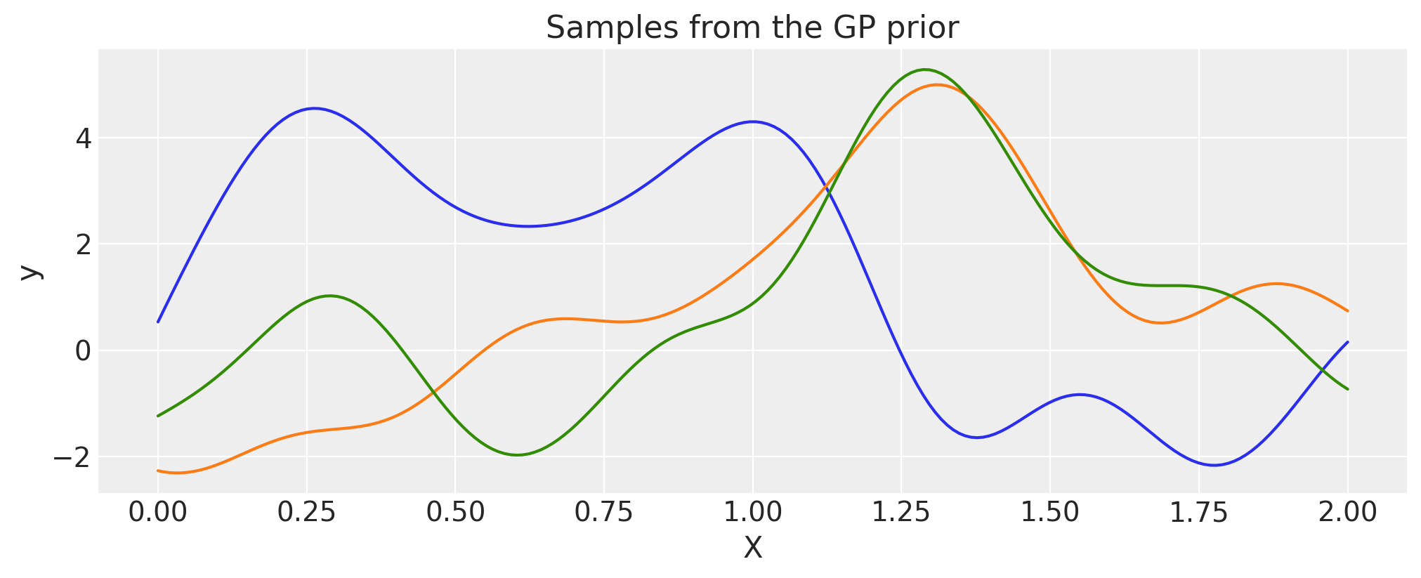
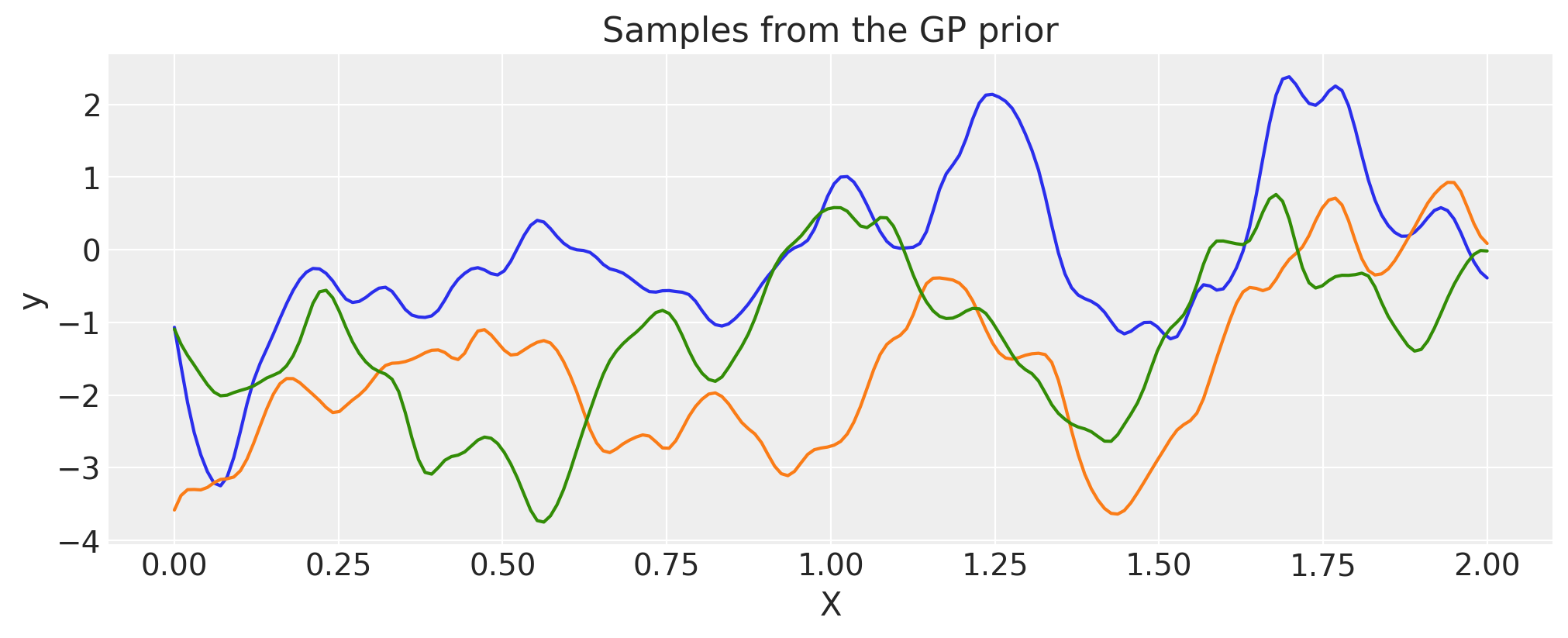
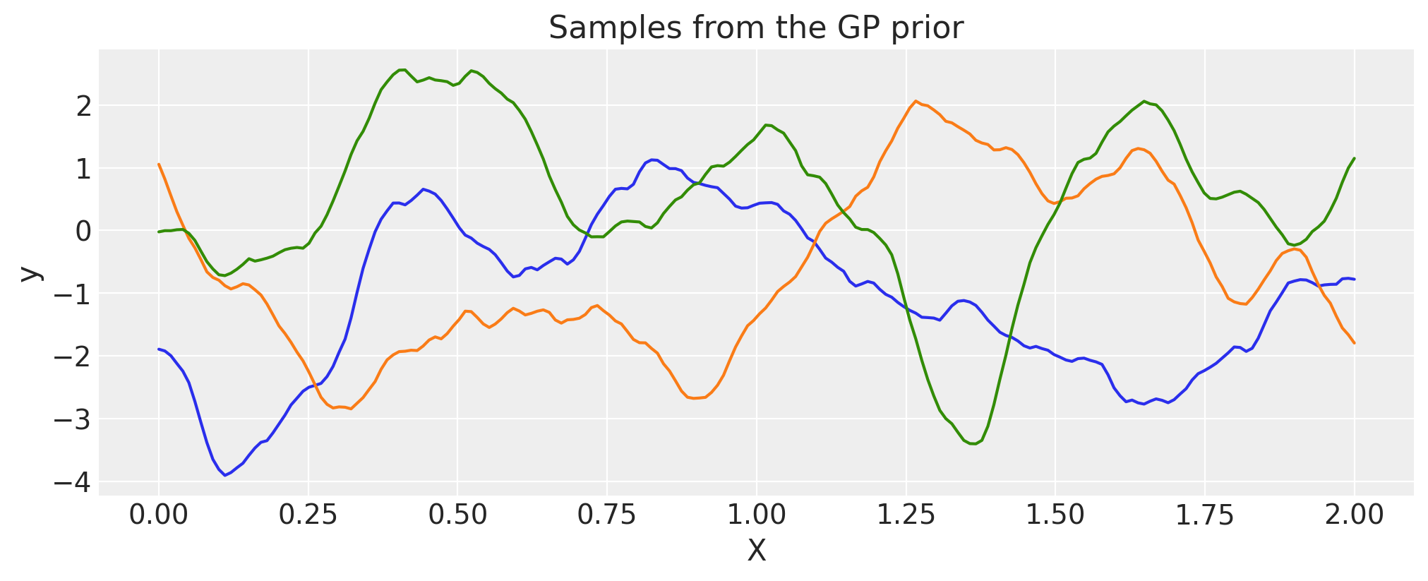
Exponentiated Quadratic#

\[ k(x, x') = \mathrm{exp}\left[ -\frac{(x - x')^2}{2 \ell^2} \right] \]

lengthscale = 0.2
eta = 2.0
cov = eta**2 * pm.gp.cov.ExpQuad(1, lengthscale)
# Add white noise to stabilise
cov += pm.gp.cov.WhiteNoise(1e-6)

X = np.linspace(0, 2, 200)[:, None]
K = cov(X).eval()

plt.plot(
    X,
    pm.draw(
        pm.MvNormal.dist(mu=np.zeros(len(K)), cov=K, shape=K.shape[0]), draws=3, random_seed=rng
    ).T,
)
plt.title("Samples from the GP prior")
plt.ylabel("y")
plt.xlabel("X");

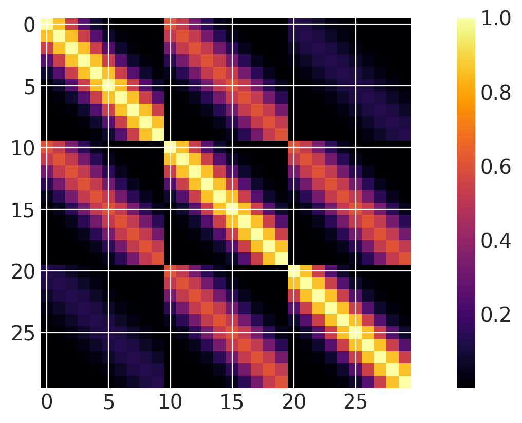
../_images/b32dad0edc3b59a6dc6f0da44044b002c11ab9c4e4995b8158637bd766cfad51.png

Two (and higher) Dimensional Inputs#

Both dimensions active#

It is easy to define kernels with higher dimensional inputs. Notice that the ls (lengthscale) parameter is an array of length 2. Lists of PyMC random variables can be used for automatic relevance determination (ARD).

x1 = np.linspace(0, 1, 10)
x2 = np.arange(1, 4)
# Cartesian product
X2 = np.dstack(np.meshgrid(x1, x2)).reshape(-1, 2)

ls = np.array([0.2, 1.0])
cov = pm.gp.cov.ExpQuad(input_dim=2, ls=ls)

m = plt.imshow(cov(X2).eval(), cmap="inferno", interpolation="none")
plt.colorbar(m);

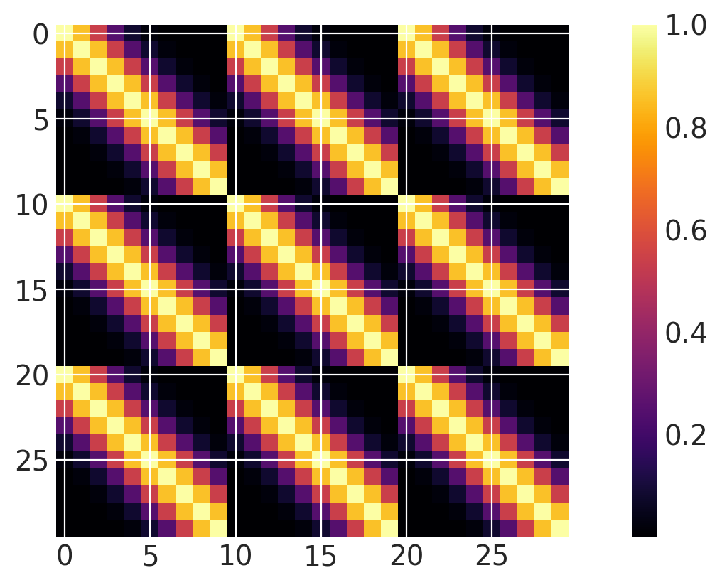
../_images/02929fba768b922f0db9de2c1599cbcdd4f1625cc961098d57c172b5ca2ee514.png

One dimension active#

ls = 0.2
cov = pm.gp.cov.ExpQuad(input_dim=2, ls=ls, active_dims=[0])

m = plt.imshow(cov(X2).eval(), cmap="inferno", interpolation="none")
plt.colorbar(m);

../_images/12b97e2a173a6b128fea67ff752b04bab1c8917cc633ba568ae432d047d6e3d4.png

Product of covariances over different dimensions#

Note that this is equivalent to using a two dimensional ExpQuad with separate lengthscale parameters for each dimension.

ls1 = 0.2
ls2 = 1.0
cov1 = pm.gp.cov.ExpQuad(2, ls1, active_dims=[0])
cov2 = pm.gp.cov.ExpQuad(2, ls2, active_dims=[1])
cov = cov1 * cov2

m = plt.imshow(cov(X2).eval(), cmap="inferno", interpolation="none")
plt.colorbar(m);

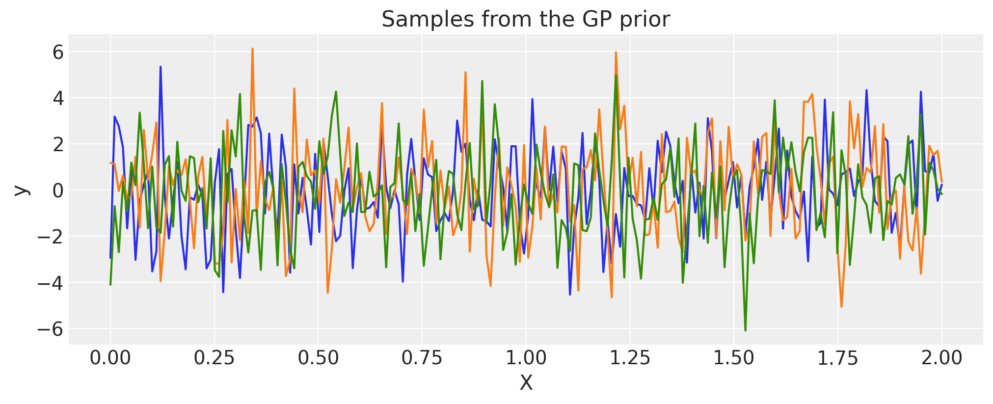
White Noise#

\[ k(x, x') = \sigma^2 \mathrm{I}_{xx} \]

sigma = 2.0
cov = pm.gp.cov.WhiteNoise(sigma)

X = np.linspace(0, 2, 200)[:, None]
K = cov(X).eval()

plt.plot(
    X,
    pm.draw(pm.MvNormal.dist(mu=np.zeros(len(K)), cov=K, shape=len(K)), draws=3, random_seed=rng).T,
)
plt.title("Samples from the GP prior")
plt.ylabel("y")
plt.xlabel("X");

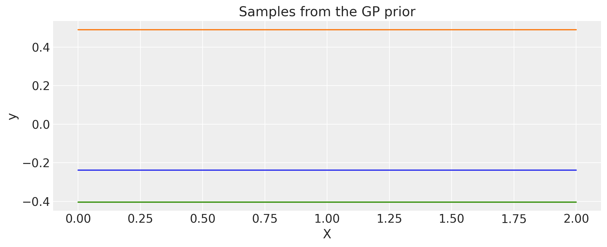
../_images/500414d8ae4ba779eda2be5fe1788a15b72a13b3f8d284a2e1cd93726b5c8a79.png

Constant#

\[ k(x, x') = c \]

c = 2.0
cov = pm.gp.cov.Constant(c)

X = np.linspace(0, 2, 200)[:, None]
K = cov(X).eval()

plt.plot(
    X,
    pm.draw(pm.MvNormal.dist(mu=np.zeros(len(K)), cov=K, shape=len(K)), draws=3, random_seed=rng).T,
)
plt.title("Samples from the GP prior")
plt.ylabel("y")
plt.xlabel("X");

../_images/6f4a4b018ef99b0c5d2d040a12203f609e8f2fa6ac7474638ac4384cf493d374.png

Rational Quadratic#

\[ k(x, x') = \left(1 + \frac{(x - x')^2}{2\alpha\ell^2} \right)^{-\alpha} \]

alpha = 0.1
ls = 0.2
tau = 2.0
cov = tau * pm.gp.cov.RatQuad(1, ls, alpha)

X = np.linspace(0, 2, 200)[:, None]
K = cov(X).eval()

plt.plot(
    X,
    pm.draw(pm.MvNormal.dist(mu=np.zeros(len(K)), cov=K, shape=len(K)), draws=3, random_seed=rng).T,
)
plt.title("Samples from the GP prior")
plt.ylabel("y")
plt.xlabel("X");

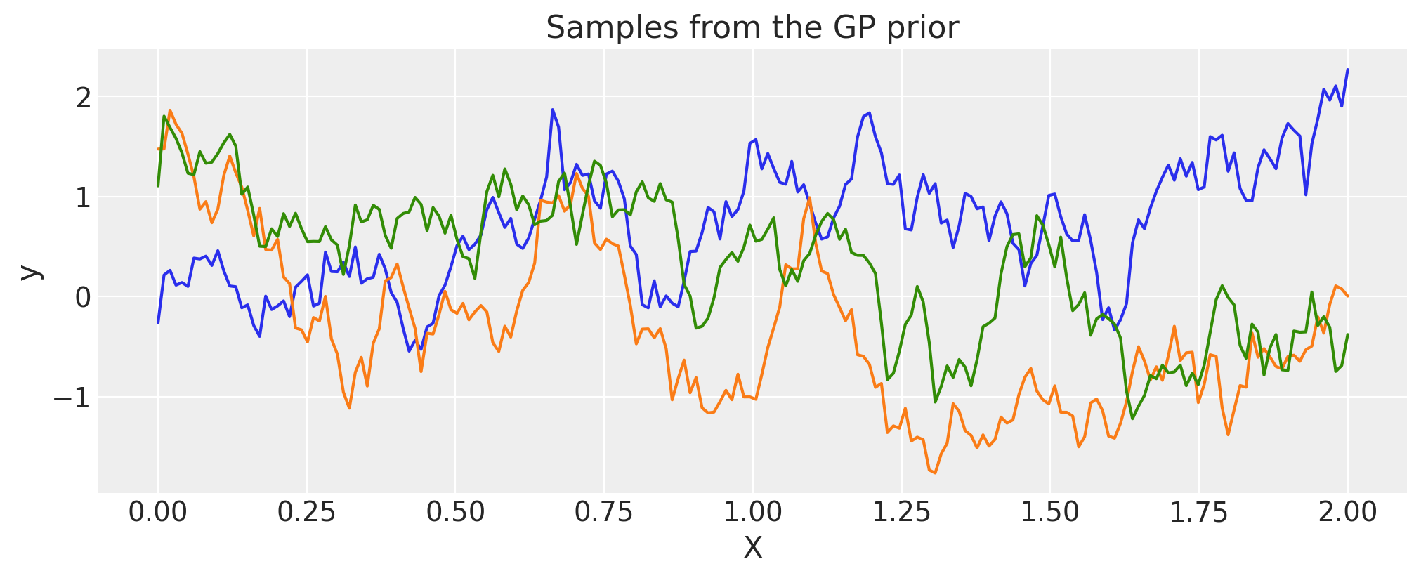
../_images/d6f8b1dd0fa3fae3925caa95e92e51ea502f3b29c71184a0316fead2a3529f30.png

Exponential#

\[ k(x, x') = \mathrm{exp}\left[ -\frac{||x - x'||}{2\ell^2} \right] \]

inverse_lengthscale = 5
cov = pm.gp.cov.Exponential(1, ls_inv=inverse_lengthscale)

X = np.linspace(0, 2, 200)[:, None]
K = cov(X).eval()

plt.plot(
    X,
    pm.draw(pm.MvNormal.dist(mu=np.zeros(len(K)), cov=K, shape=len(K)), draws=3, random_seed=rng).T,
)
plt.title("Samples from the GP prior")
plt.ylabel("y")
plt.xlabel("X");

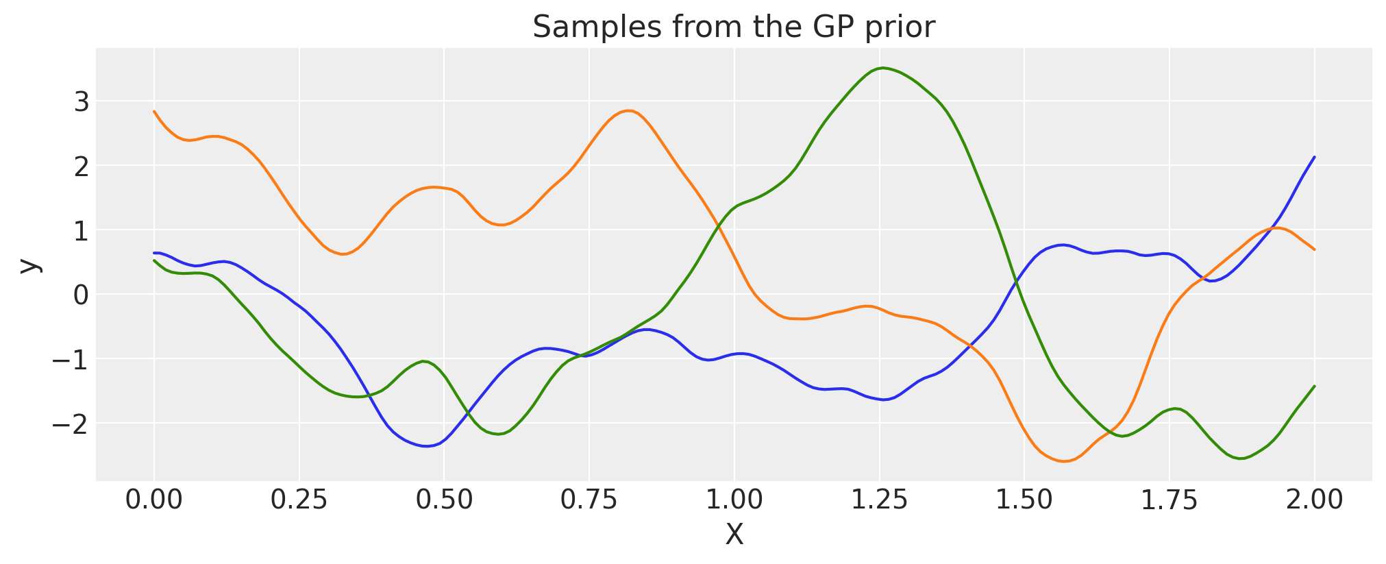
../_images/5ea3b84aa82fe06fcb7c54511531c3fc18739f82629a05057f90b60fcf1a83d0.png

Matern 5/2#

\[ k(x, x') = \left(1 + \frac{\sqrt{5(x - x')^2}}{\ell} + \frac{5(x-x')^2}{3\ell^2}\right) \mathrm{exp}\left[ - \frac{\sqrt{5(x - x')^2}}{\ell} \right] \]

ls = 0.2
tau = 2.0
cov = tau * pm.gp.cov.Matern52(1, ls)

X = np.linspace(0, 2, 200)[:, None]
K = cov(X).eval()

plt.plot(
    X,
    pm.draw(pm.MvNormal.dist(mu=np.zeros(len(K)), cov=K, shape=len(K)), draws=3, random_seed=rng).T,
)
plt.title("Samples from the GP prior")
plt.ylabel("y")
plt.xlabel("X");

../_images/1b345944b2480a075afffbe317e1defb18629231e0f1ead08ecfa45fd8aefcc9.png

Matern 3/2#

\[ k(x, x') = \left(1 + \frac{\sqrt{3(x - x')^2}}{\ell}\right) \mathrm{exp}\left[ - \frac{\sqrt{3(x - x')^2}}{\ell} \right] \]

ls = 0.2
tau = 2.0
cov = tau * pm.gp.cov.Matern32(1, ls)

X = np.linspace(0, 2, 200)[:, None]
K = cov(X).eval()

plt.plot(
    X,
    pm.draw(pm.MvNormal.dist(mu=np.zeros(len(K)), cov=K, shape=len(K)), draws=3, random_seed=rng).T,
)
plt.title("Samples from the GP prior")
plt.ylabel("y")
plt.xlabel("X");

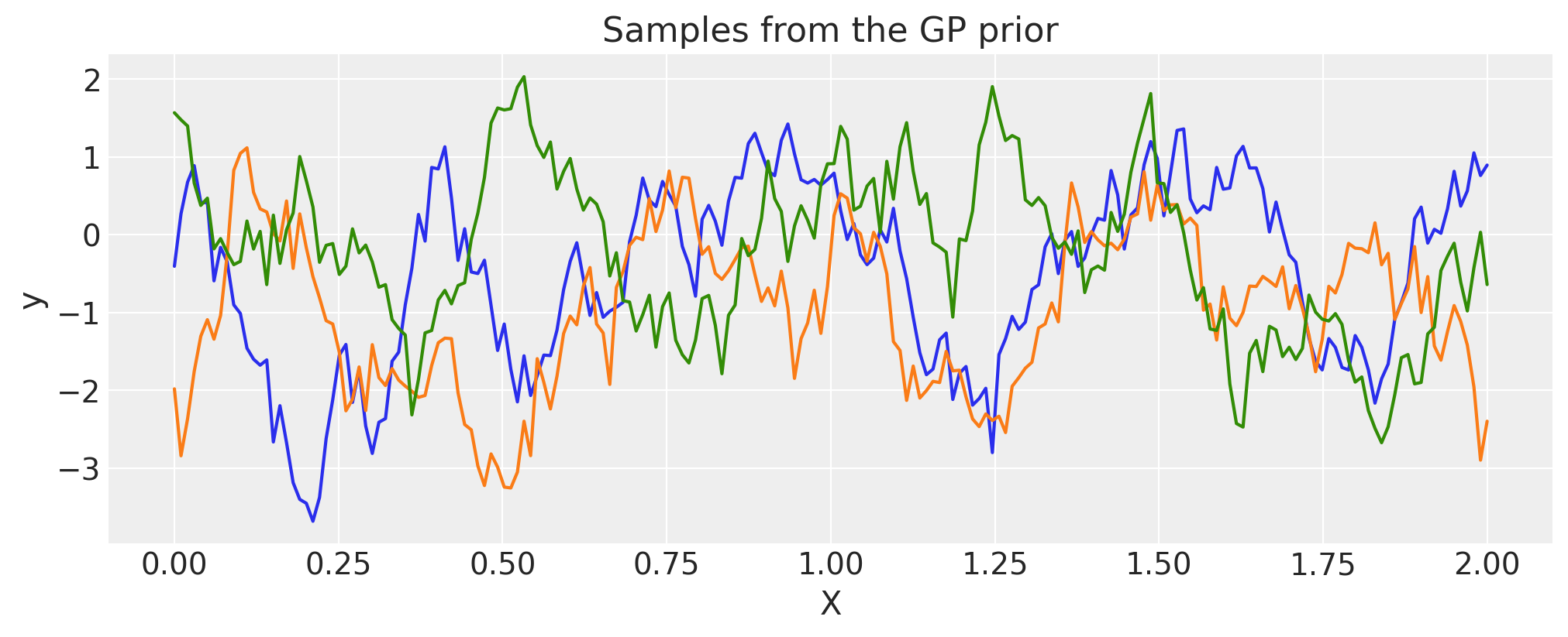
../_images/8f165b1cd6e165553793e18b94fcedc6ee6a879963dcc0a889a740a92449099d.png

Matern 1/2#

\[k(x, x') = \mathrm{exp}\left[ -\frac{(x - x')^2}{\ell} \right]\]

ls = 0.2
tau = 2.0
cov = tau * pm.gp.cov.Matern12(1, ls)

X = np.linspace(0, 2, 200)[:, None]
K = cov(X).eval()

plt.plot(
    X,
    pm.draw(pm.MvNormal.dist(mu=np.zeros(len(K)), cov=K, shape=len(K)), draws=3, random_seed=rng).T,
)
plt.title("Samples from the GP prior")
plt.ylabel("y")
plt.xlabel("X");

../_images/ed76843d12dfd9f1db980d4daf441fc6555706b75a2627a32e83124a8bbc8bfa.png

Cosine#

\[ k(x, x') = \mathrm{cos}\left( 2 \pi \frac{||x - x'||}{ \ell^2} \right) \]

period = 0.5
cov = pm.gp.cov.Cosine(1, period)
# Add white noise to stabilise
cov += pm.gp.cov.WhiteNoise(1e-4)

X = np.linspace(0, 2, 200)[:, None]
K = cov(X).eval()

plt.plot(
    X,
    pm.draw(pm.MvNormal.dist(mu=np.zeros(len(K)), cov=K, shape=len(K)), draws=3, random_seed=rng).T,
)
plt.title("Samples from the GP prior")
plt.ylabel("y")
plt.xlabel("X");

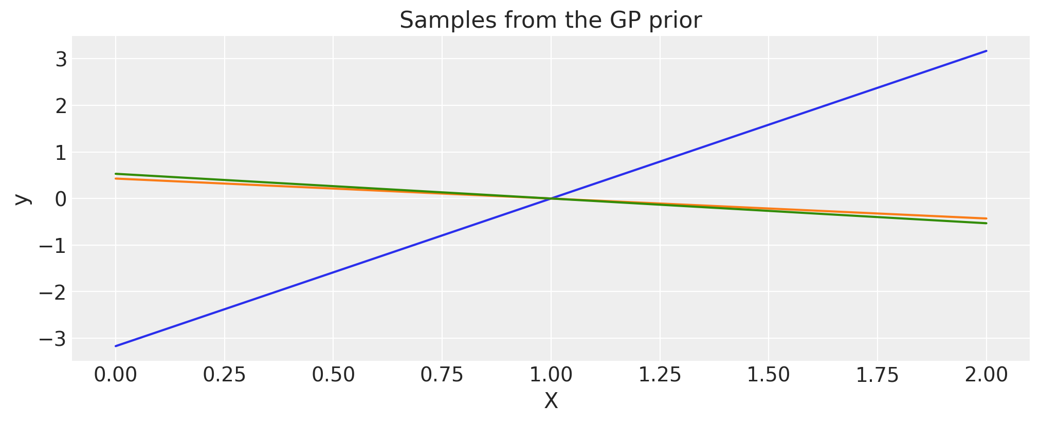
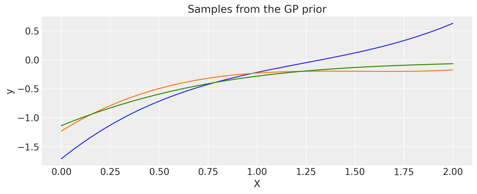
../_images/8e4787d3f82349aef3c5df155d63317fa1c1e353c4f87a0579689406a21d15fd.png

Linear#

\[ k(x, x') = (x - c)(x' - c) \]

c = 1.0
tau = 2.0
cov = tau * pm.gp.cov.Linear(1, c)
# Add white noise to stabilise
cov += pm.gp.cov.WhiteNoise(1e-6)

X = np.linspace(0, 2, 200)[:, None]
K = cov(X).eval()

plt.plot(
    X,
    pm.draw(pm.MvNormal.dist(mu=np.zeros(len(K)), cov=K, shape=len(K)), draws=3, random_seed=rng).T,
)
plt.title("Samples from the GP prior")
plt.ylabel("y")
plt.xlabel("X");

../_images/c90bfbfc82b41ed9b678970725e9f9bf9fa471bf1e1f0307efb2c5d559691747.png

Polynomial#

\[ k(x, x') = [(x - c)(x' - c) + \mathrm{offset}]^{d} \]

c = 1.0
d = 3
offset = 1.0
tau = 0.1
cov = tau * pm.gp.cov.Polynomial(1, c=c, d=d, offset=offset)
# Add white noise to stabilise
cov += pm.gp.cov.WhiteNoise(1e-6)

X = np.linspace(0, 2, 200)[:, None]
K = cov(X).eval()

plt.plot(
    X,
    pm.draw(pm.MvNormal.dist(mu=np.zeros(len(K)), cov=K, shape=len(K)), draws=3, random_seed=rng).T,
)
plt.title("Samples from the GP prior")
plt.ylabel("y")
plt.xlabel("X");

../_images/d8cd362b8bce0e258bba3116453249c4ebc4099f8d5cfaff84d7096a5b85425e.png

Multiplication with a precomputed covariance matrix#

A covariance function cov can be multiplied with numpy matrix, K_cos, as long as the shapes are appropriate.

# first evaluate a covariance function into a matrix
period = 0.2
cov_cos = pm.gp.cov.Cosine(1, period)
K_cos = cov_cos(X).eval()

# now multiply it with a covariance *function*
cov = pm.gp.cov.Matern32(1, 0.5) * K_cos

X = np.linspace(0, 2, 200)[:, None]
K = cov(X).eval()

plt.plot(
    X,
    pm.draw(pm.MvNormal.dist(mu=np.zeros(len(K)), cov=K, shape=len(K)), draws=3, random_seed=rng).T,
)
plt.title("Samples from the GP prior")
plt.ylabel("y")
plt.xlabel("X");

../_images/360b5f89d07006361219bcc2b9b44c12f81cba8c4f0cf05df1f2a82a6e18f130.png

Applying an arbitrary warping function on the inputs#

If \(k(x, x')\) is a valid covariance function, then so is \(k(w(x), w(x'))\).

The first argument of the warping function must be the input X. The remaining arguments can be anything else, including random variables.

def warp_func(x, a, b, c):
    return 1.0 + x + (a * pt.tanh(b * (x - c)))


a = 1.0
b = 5.0
c = 1.0

cov_exp = pm.gp.cov.ExpQuad(1, 0.2)
cov = pm.gp.cov.WarpedInput(1, warp_func=warp_func, args=(a, b, c), cov_func=cov_exp)
# Add white noise to stabilise
cov += pm.gp.cov.WhiteNoise(1e-6)

X = np.linspace(0, 2, 400)[:, None]
wf = warp_func(X.flatten(), a, b, c).eval()

plt.plot(X, wf)
plt.xlabel("X")
plt.ylabel("warp_func(X)")
plt.title("The warping function used")

K = cov(X).eval()
plt.plot(
    X,
    pm.draw(pm.MvNormal.dist(mu=np.zeros(len(K)), cov=K, shape=len(K)), draws=3, random_seed=rng).T,
)
plt.title("Samples from the GP prior")
plt.ylabel("y")
plt.xlabel("X");

../_images/42d54c0850a3fad919c28143f8fab6978d27e2c45203c8bbc81673a54231de2f.png

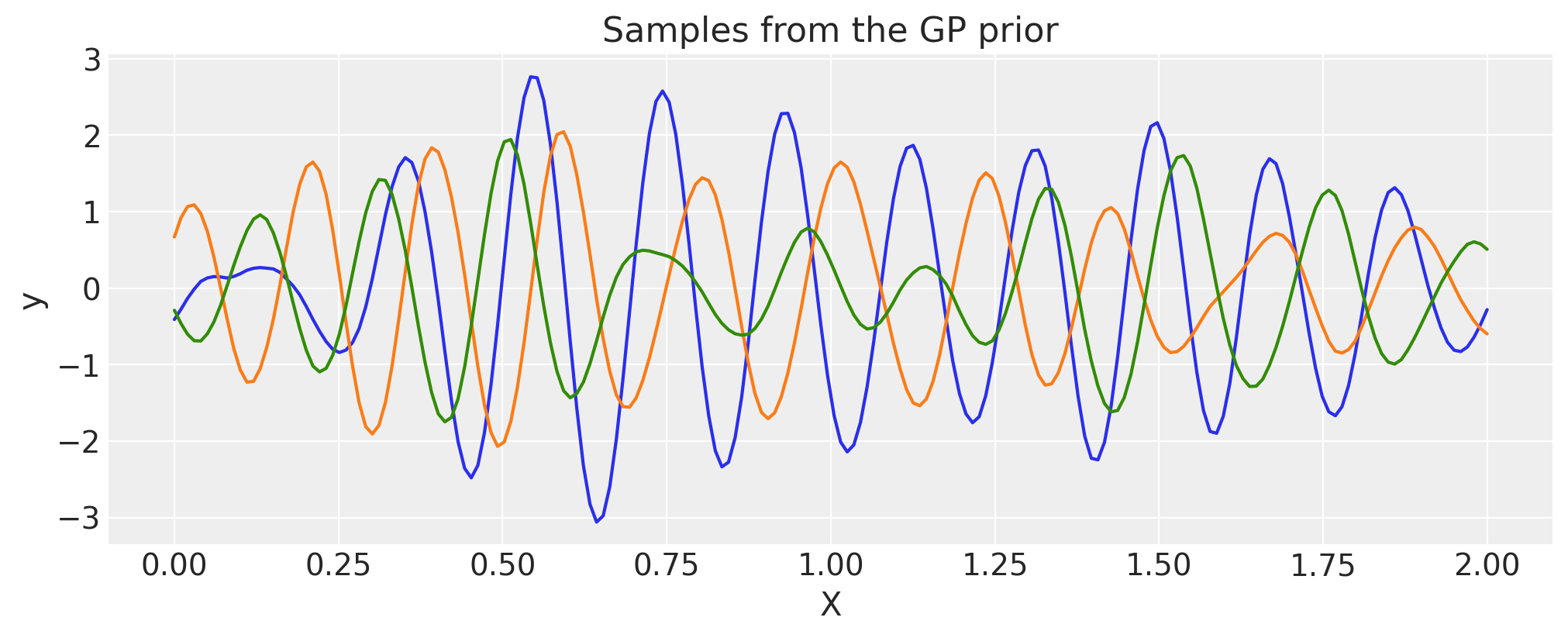
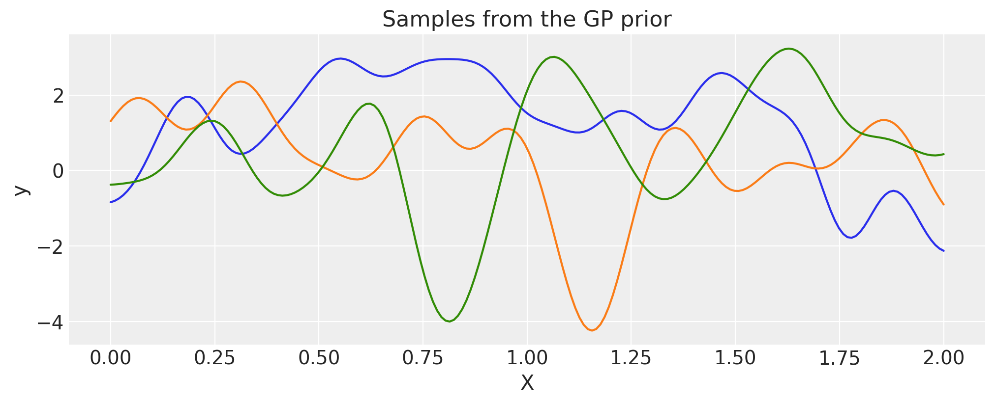
Constructing `Periodic` using `WarpedInput`#

The WarpedInput kernel can be used to create the Periodic covariance. This covariance models functions that are periodic, but are not an exact sine wave (like the Cosine kernel is).

The periodic kernel is given by

\[ k(x, x') = \exp\left( -\frac{2 \sin^{2}(\pi |x - x'|\frac{1}{T})}{\ell^2} \right) \]

Where T is the period, and \(\ell\) is the lengthscale. It can be derived by warping the input of an ExpQuad kernel with the function \(\mathbf{u}(x) = (\sin(2\pi x \frac{1}{T})\,, \cos(2 \pi x \frac{1}{T}))\). Here we use the WarpedInput kernel to construct it.

The input X, which is defined at the top of this page, is 2 “seconds” long. We use a period of \(0.5\), which means that functions drawn from this GP prior will repeat 4 times over 2 seconds.

def mapping(x, T):
    c = 2.0 * np.pi * (1.0 / T)
    u = pt.concatenate((pt.sin(c * x), pt.cos(c * x)), 1)
    return u


T = 0.6
ls = 0.4
# note that the input of the covariance function taking
#    the inputs is 2 dimensional
cov_exp = pm.gp.cov.ExpQuad(2, ls)
cov = pm.gp.cov.WarpedInput(1, cov_func=cov_exp, warp_func=mapping, args=(T,))
# Add white noise to stabilise
cov += pm.gp.cov.WhiteNoise(1e-6)

K = cov(X).eval()
plt.plot(
    X,
    pm.draw(pm.MvNormal.dist(mu=np.zeros(len(K)), cov=K, shape=len(K)), draws=3, random_seed=rng).T,
)
plt.title("Samples from the GP prior")
plt.ylabel("y")
plt.xlabel("X");

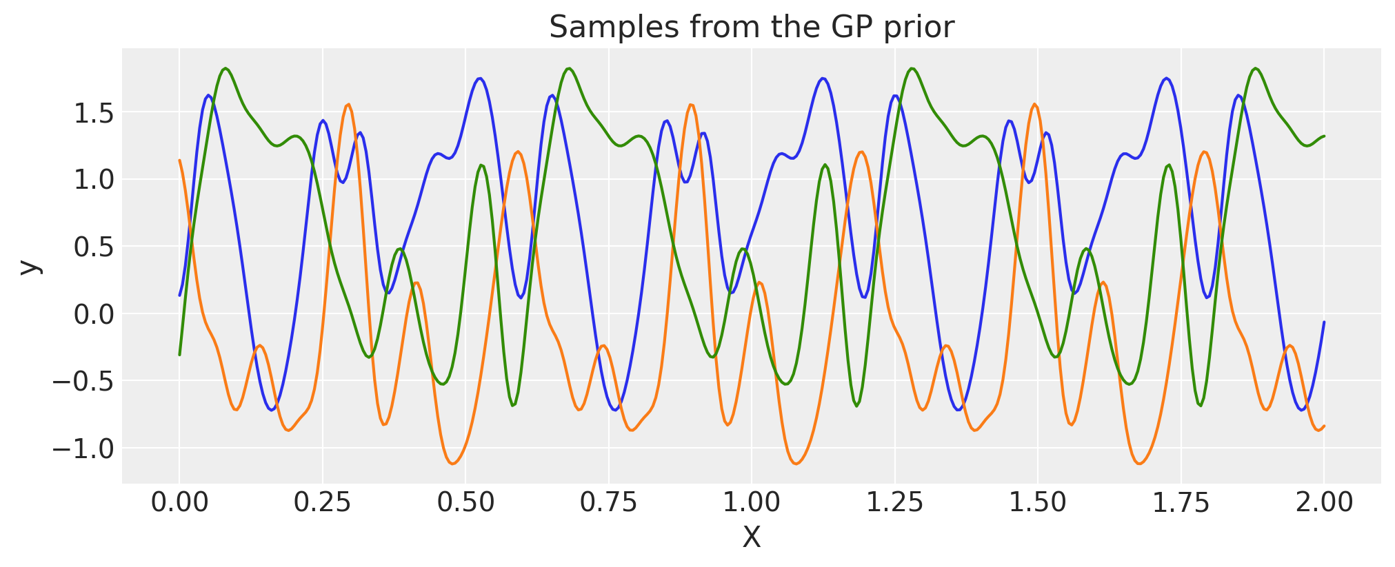
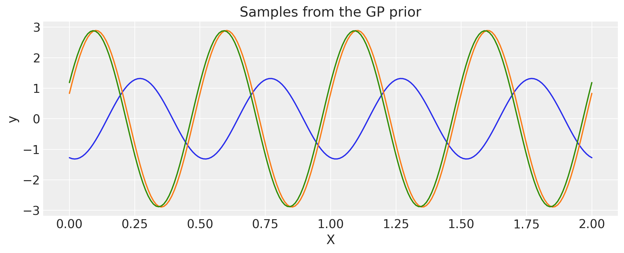
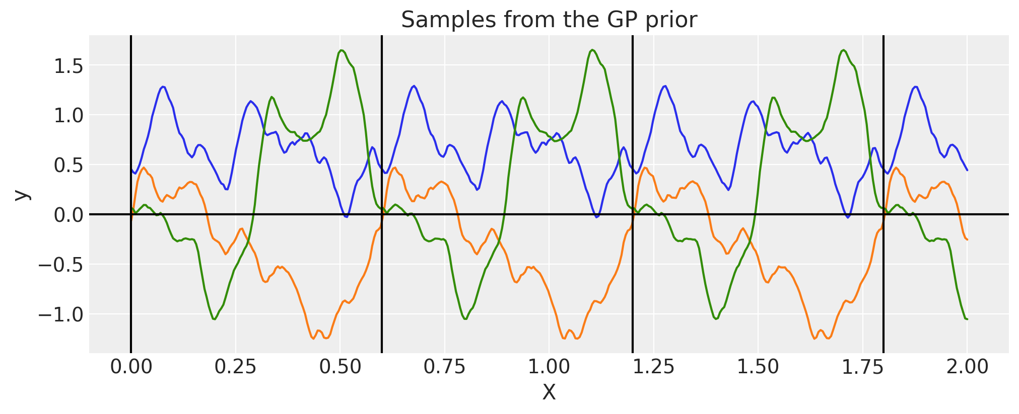
../_images/e1c313af0269301db4d821ea64cc4b375b2f562bd104310e9581235180048724.png

Periodic#

There is no need to construct the periodic covariance this way every time. A more efficient implementation of this covariance function is built in.

period = 0.6
ls = 0.4
cov = pm.gp.cov.Periodic(1, period=period, ls=ls)
# Add white noise to stabilise
cov += pm.gp.cov.WhiteNoise(1e-6)

K = cov(X).eval()
plt.plot(
    X,
    pm.draw(pm.MvNormal.dist(mu=np.zeros(len(K)), cov=K, shape=len(K)), draws=3, random_seed=rng).T,
)
for p in np.arange(0, 2, period):
    plt.axvline(p, color="black")
plt.axhline(0, color="black")
plt.title("Samples from the GP prior")
plt.ylabel("y")
plt.xlabel("X");

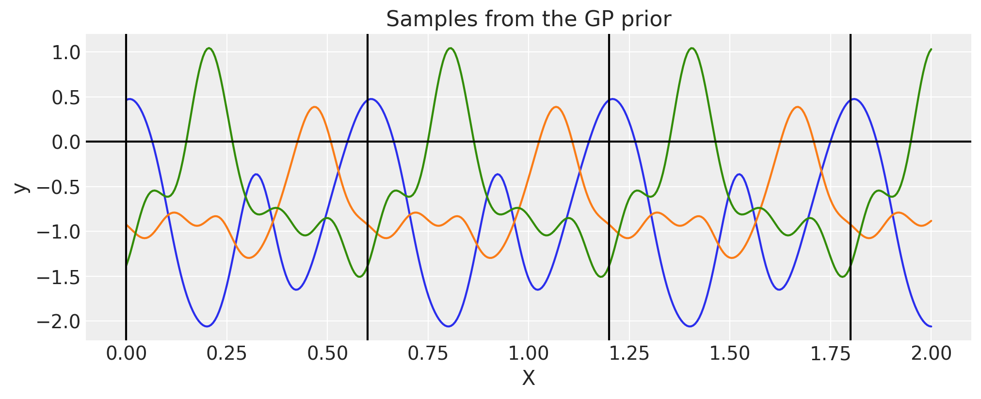
../_images/40eaca259ebda4a81144fdc7b28d37d0c8ba38e49bbd593e54f15e325be00715.png

Circular#

Circular kernel is similar to Periodic one but has an additional nuisance parameter \(\tau\)

In Padonou and Roustant [2015], the Weinland function is used to solve the problem and ensures positive definite kernel on the circular domain (and not only).

\[ W_c(t) = \left(1 + \tau \frac{t}{c}\right)\left(1-\frac{t}{c}\right)_+^\tau \]

where \(c\) is maximum value for \(t\) and \(\tau\ge 4\) is some positive number

The kernel itself for geodesic distance (arc length) on a circle looks like

\[ k_g(x, y) = W_\pi(\text{dist}_{\mathit{geo}}(x, y)) \]

Briefly, you can think

\(t\) is time, it runs from \(0\) to \(24\) and then goes back to \(0\)
\(c\) is maximum distance between any timestamps, here it would be \(12\)
\(\tau\) controls for correlation strength, larger \(\tau\) leads to less smooth functions

period = 0.6
tau = 4
cov = pm.gp.cov.Circular(1, period=period, tau=tau)

K = cov(X).eval()
plt.plot(
    X,
    pm.draw(pm.MvNormal.dist(mu=np.zeros(len(K)), cov=K, shape=len(K)), draws=3, random_seed=rng).T,
)
for p in np.arange(0, 2, period):
    plt.axvline(p, color="black")
plt.axhline(0, color="black")
plt.title("Samples from the GP prior")
plt.ylabel("y")
plt.xlabel("X");

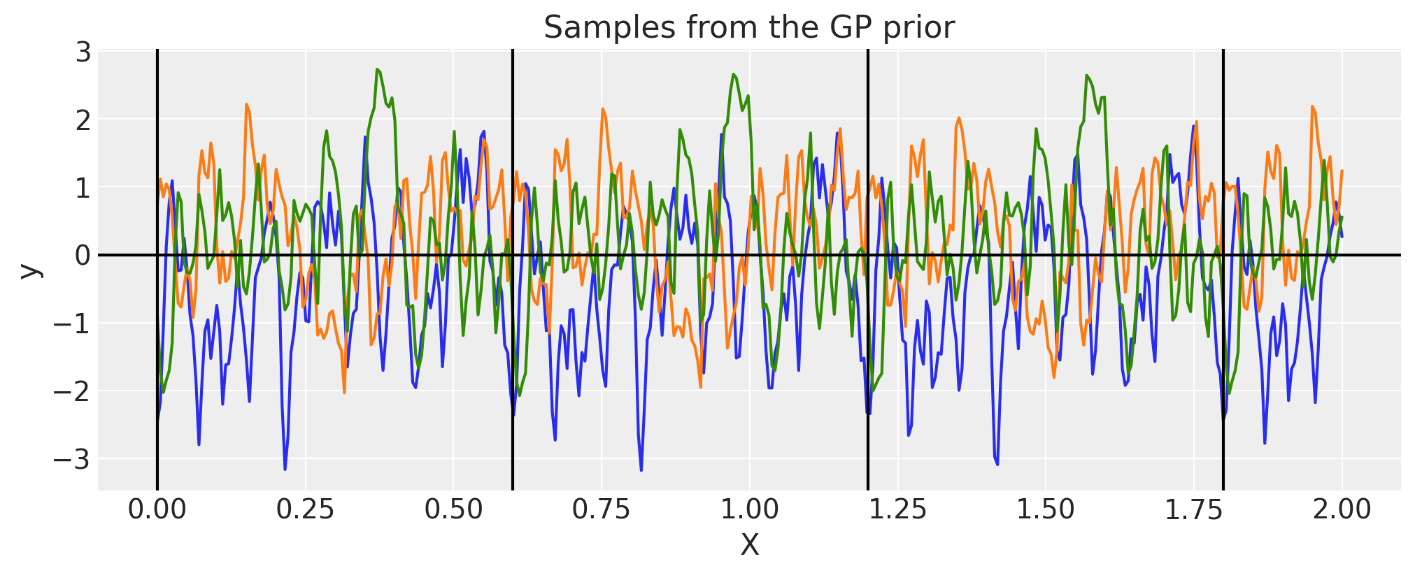
../_images/019d297f79d0a03d83aee6e4c1202c5ef63d3b168d97dffd6b19fe5609df721a.png

We can see the effect of \(\tau\), it adds more non-smooth patterns

period = 0.6
tau = 40
cov = pm.gp.cov.Circular(1, period=period, tau=tau)

K = cov(X).eval()
plt.plot(
    X,
    pm.draw(pm.MvNormal.dist(mu=np.zeros(len(K)), cov=K, shape=len(K)), draws=3, random_seed=rng).T,
)
for p in np.arange(0, 2, period):
    plt.axvline(p, color="black")
plt.axhline(0, color="black")
plt.title("Samples from the GP prior")
plt.ylabel("y")
plt.xlabel("X");

../_images/8e9975ae80a3ea7ff3779c9832f7f07a1f62db433c8b4317428db5e7f2c64606.png

Gibbs#

The Gibbs covariance function applies a positive definite warping function to the lengthscale. Similarly to WarpedInput, the lengthscale warping function can be specified with parameters that are either fixed or random variables.

def tanh_func(x, ls1, ls2, w, x0):
    """
    ls1: left saturation value
    ls2: right saturation value
    w:   transition width
    x0:  transition location.
    """
    return (ls1 + ls2) / 2.0 - (ls1 - ls2) / 2.0 * pt.tanh((x - x0) / w)


ls1 = 0.05
ls2 = 0.6
w = 0.3
x0 = 1.0
cov = pm.gp.cov.Gibbs(1, tanh_func, args=(ls1, ls2, w, x0))
# Add white noise to stabilise
cov += pm.gp.cov.WhiteNoise(1e-6)

wf = tanh_func(X, ls1, ls2, w, x0).eval()
plt.plot(X, wf)
plt.ylabel("lengthscale")
plt.xlabel("X")
plt.title("Lengthscale as a function of X")

K = cov(X).eval()
plt.plot(
    X,
    pm.draw(pm.MvNormal.dist(mu=np.zeros(len(K)), cov=K, shape=len(K)), draws=3, random_seed=rng).T,
)
plt.title("Samples from the GP prior")
plt.ylabel("y")
plt.xlabel("X");

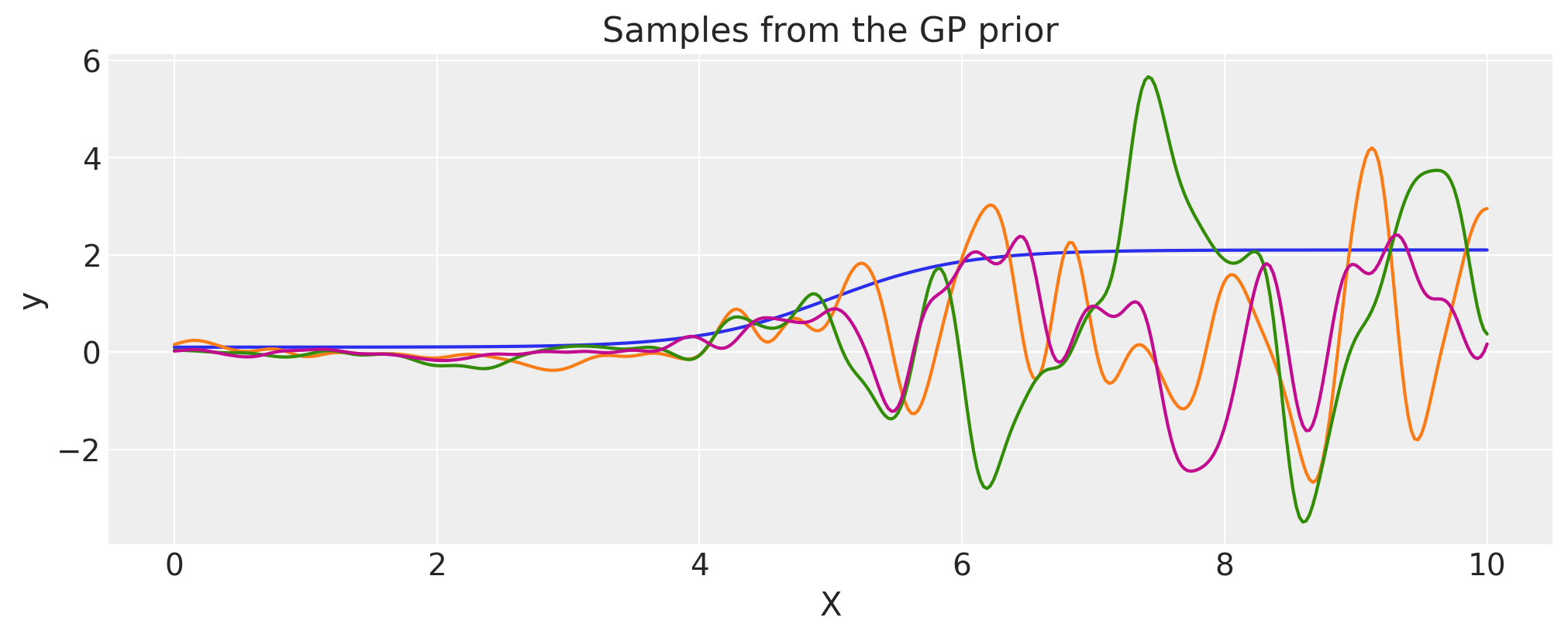
../_images/8b00c9a743465c012b12bb8a9b1cc7078f7d31fd77b5af2752fcc4226c3910ba.png

Scaled Covariance#

One can construct a new kernel or covariance function by multiplying some base kernel by a nonnegative function \(\phi(x)\),

\[ k_{\mathrm{scaled}}(x, x') = \phi(x) k_{\mathrm{base}}(x, x') \phi(x') \,. \]

This is useful for specifying covariance functions whose amplitude changes across the domain.

def logistic(x, a, x0, c, d):
    # a is the slope, x0 is the location
    return d * pm.math.invlogit(a * (x - x0)) + c


a = 2.0
x0 = 5.0
c = 0.1
d = 2.0

cov_base = pm.gp.cov.ExpQuad(1, 0.2)
cov = pm.gp.cov.ScaledCov(1, scaling_func=logistic, args=(a, x0, c, d), cov_func=cov_base)
# Add white noise to stabilise
cov += pm.gp.cov.WhiteNoise(1e-5)

X = np.linspace(0, 10, 400)[:, None]
lfunc = logistic(X.flatten(), a, b, c, d).eval()

plt.plot(X, lfunc)
plt.xlabel("X")
plt.ylabel(r"$\phi(x)$")
plt.title("The scaling function")

K = cov(X).eval()
plt.plot(
    X,
    pm.draw(pm.MvNormal.dist(mu=np.zeros(len(K)), cov=K, shape=len(K)), draws=3, random_seed=rng).T,
)
plt.title("Samples from the GP prior")
plt.ylabel("y")
plt.xlabel("X");

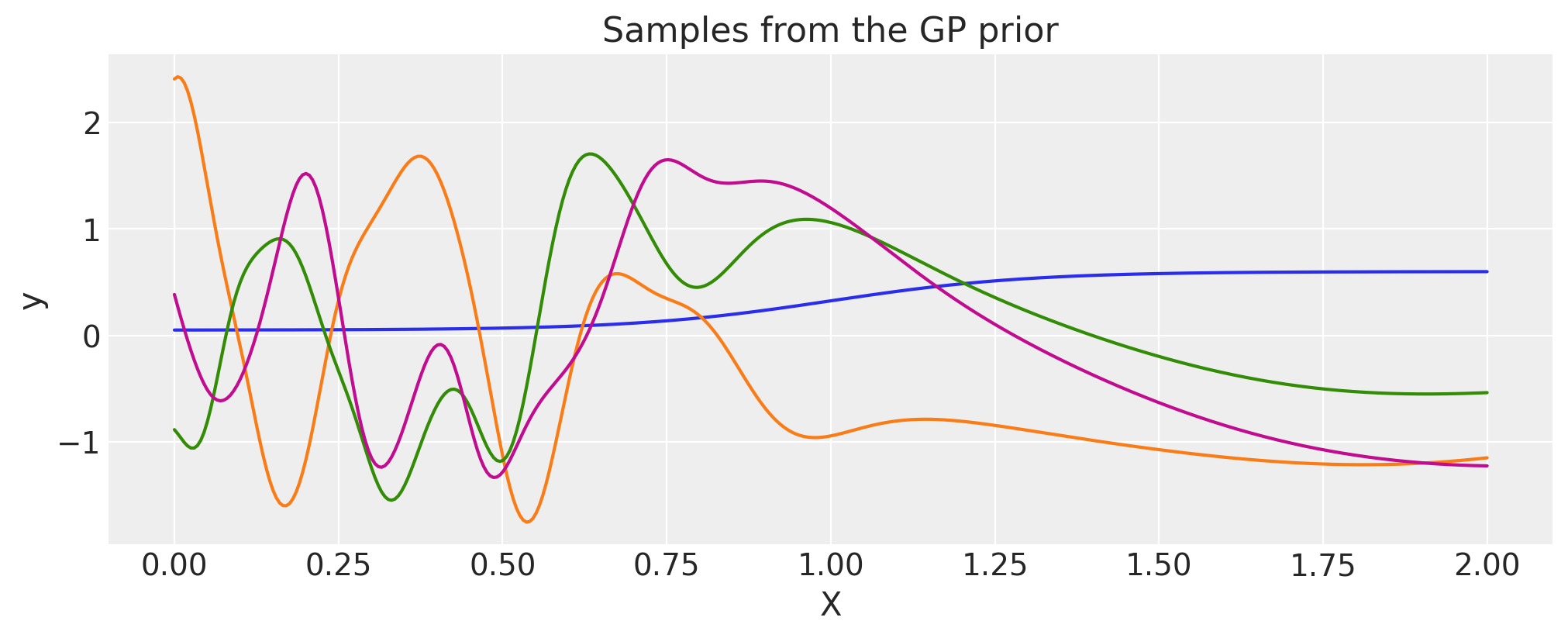
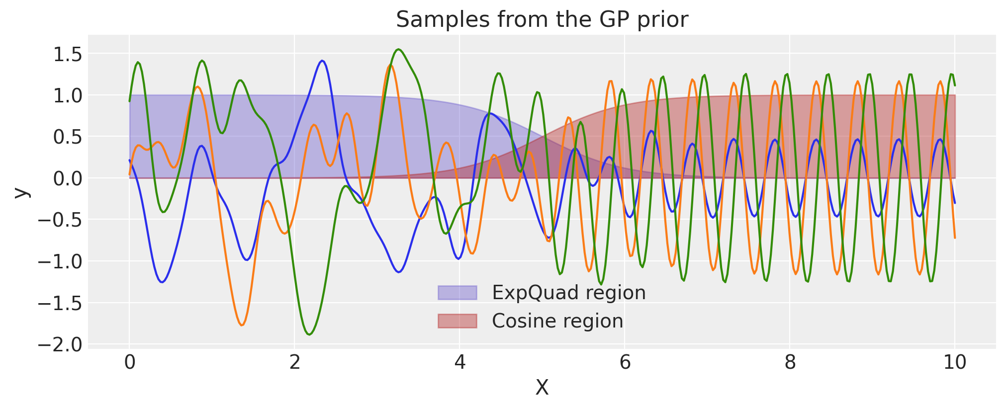
../_images/dd3acd30c7c9867a0a04ebcac57618386506ec3b892b3ef10a90632aaa2b4ff4.png

Constructing a Changepoint kernel using `ScaledCov`#

The ScaledCov kernel can be used to create the Changepoint covariance. This covariance models a process that gradually transitions from one type of behavior to another.

The changepoint kernel is given by

\[ k(x, x') = \phi(x)k_{1}(x, x')\phi(x) + (1 - \phi(x))k_{2}(x, x')(1 - \phi(x')) \]

where \(\phi(x)\) is the logistic function.

def logistic(x, a, x0):
    # a is the slope, x0 is the location
    return pm.math.invlogit(a * (x - x0))


a = 2.0
x0 = 5.0

cov1 = pm.gp.cov.ScaledCov(
    1, scaling_func=logistic, args=(-a, x0), cov_func=pm.gp.cov.ExpQuad(1, 0.2)
)
cov2 = pm.gp.cov.ScaledCov(
    1, scaling_func=logistic, args=(a, x0), cov_func=pm.gp.cov.Cosine(1, 0.5)
)
cov = cov1 + cov2
# Add white noise to stabilise
cov += pm.gp.cov.WhiteNoise(1e-5)

X = np.linspace(0, 10, 400)
plt.fill_between(
    X,
    np.zeros(400),
    logistic(X, -a, x0).eval(),
    label="ExpQuad region",
    color="slateblue",
    alpha=0.4,
)
plt.fill_between(
    X, np.zeros(400), logistic(X, a, x0).eval(), label="Cosine region", color="firebrick", alpha=0.4
)
plt.legend()
plt.xlabel("X")
plt.ylabel(r"$\phi(x)$")
plt.title("The two scaling functions")

K = cov(X[:, None]).eval()
plt.plot(
    X,
    pm.draw(pm.MvNormal.dist(mu=np.zeros(len(K)), cov=K, shape=len(K)), draws=3, random_seed=rng).T,
)
plt.title("Samples from the GP prior")
plt.ylabel("y")
plt.xlabel("X");

../_images/f46cf4b68216f30aa74278b3869e92133129d550799ea2631cf2edac64e0c4ef.png

Combination of two or more Covariance functions#

You can combine different covariance functions to model complex data.

In particular, you can perform the following operations on any covaraince functions:

Add other covariance function with equal or broadcastable dimensions with first covariance function
Multiply with a scalar or a covariance function with equal or broadcastable dimensions with first covariance function
Exponentiate with a scalar.

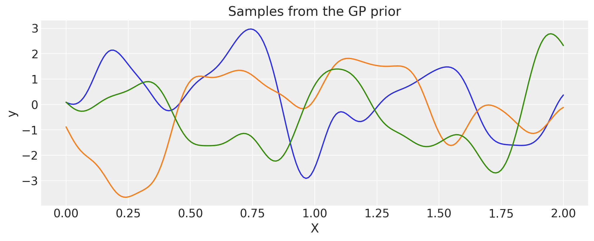
Addition#

ls_1 = 0.1
tau_1 = 2.0
ls_2 = 0.5
tau_2 = 1.0
cov_1 = tau_1 * pm.gp.cov.ExpQuad(1, ls=ls_1)
cov_2 = tau_2 * pm.gp.cov.ExpQuad(1, ls=ls_2)

cov = cov_1 + cov_2
# Add white noise to stabilise
cov += pm.gp.cov.WhiteNoise(1e-6)

X = np.linspace(0, 2, 200)[:, None]
K = cov(X).eval()

plt.plot(
    X,
    pm.draw(pm.MvNormal.dist(mu=np.zeros(len(K)), cov=K, shape=len(K)), draws=3, random_seed=rng).T,
)
plt.title("Samples from the GP prior")
plt.ylabel("y")
plt.xlabel("X");

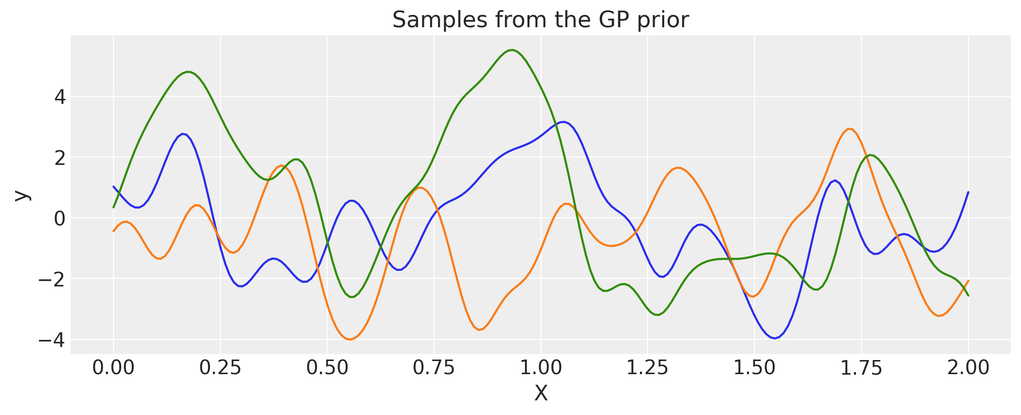
../_images/c42ce6bfaf672cce11e86735fe8c738c88dba6d70703f05adc43a2d3d54dcb76.png

Multiplication#

ls_1 = 0.1
tau_1 = 2.0
ls_2 = 0.5
tau_2 = 1.0
cov_1 = tau_1 * pm.gp.cov.ExpQuad(1, ls=ls_1)
cov_2 = tau_2 * pm.gp.cov.ExpQuad(1, ls=ls_2)

cov = cov_1 * cov_2
# Add white noise to stabilise
cov += pm.gp.cov.WhiteNoise(1e-6)

X = np.linspace(0, 2, 200)[:, None]
K = cov(X).eval()

plt.plot(
    X,
    pm.draw(pm.MvNormal.dist(mu=np.zeros(len(K)), cov=K, shape=len(K)), draws=3, random_seed=rng).T,
)
plt.title("Samples from the GP prior")
plt.ylabel("y")
plt.xlabel("X");

../_images/14a070e3680e48e0009ae52f369aea5a8280af7b09829526b89abf2a6fce0ae0.png

Exponentiation#

ls_1 = 0.1
tau_1 = 2.0
power = 2
cov_1 = tau_1 * pm.gp.cov.ExpQuad(1, ls=ls_1)

cov = cov_1**power
# Add white noise to stabilise
cov += pm.gp.cov.WhiteNoise(1e-6)

X = np.linspace(0, 2, 200)[:, None]
K = cov(X).eval()

plt.plot(
    X,
    pm.draw(pm.MvNormal.dist(mu=np.zeros(len(K)), cov=K, shape=len(K)), draws=3, random_seed=rng).T,
)
plt.title("Samples from the GP prior")
plt.ylabel("y")
plt.xlabel("X");

../_images/6c071d02ad948c36537eee48a89de646893668dd1a7ddf9e7ee4081453fe6753.png

Defining a custom covariance function#

Covariance function objects in PyMC need to implement the __init__, diag, and full methods, and subclass gp.cov.Covariance. diag returns only the diagonal of the covariance matrix, and full returns the full covariance matrix. The full method has two inputs X and Xs. full(X) returns the square covariance matrix, and full(X, Xs) returns the cross-covariances between the two sets of inputs.

For example, here is the implementation of the WhiteNoise covariance function:

class WhiteNoise(pm.gp.cov.Covariance):
    def __init__(self, sigma):
        super(WhiteNoise, self).__init__(1, None)
        self.sigma = sigma

    def diag(self, X):
        return tt.alloc(tt.square(self.sigma), X.shape[0])

    def full(self, X, Xs=None):
        if Xs is None:
            return tt.diag(self.diag(X))
        else:
            return tt.alloc(0.0, X.shape[0], Xs.shape[0])

If we have forgotten an important covariance or mean function, please feel free to submit a pull request!

References#

[1]

Carl Edward Rasmussen and Christopher K. I. Williams. Gaussian Processes for Machine Learning. The MIT Press, 2006. ISBN 026218253X. URL: https://gaussianprocess.org/gpml/.

[2]

Espéran Padonou and O Roustant. Polar Gaussian Processes for Predicting on Circular Domains. working paper or preprint, February 2015. URL: https://hal.archives-ouvertes.fr/hal-01119942.

Authors#

Authored by Bill Engels
Updated to v4 by Oriol Abril Pla in Nov 2022 (pymc-examples#301)
Updated to v5 by Juan Orduz in Nov 2023 (pymc-examples#593)

Watermark#

%load_ext watermark
%watermark -n -u -v -iv -w -p xarray

Last updated: Fri Nov 17 2023

Python implementation: CPython
Python version       : 3.11.5
IPython version      : 8.17.2

xarray: 2023.10.1

matplotlib: 3.8.1
arviz     : 0.16.1
pymc      : 5.9.2
pytensor  : 2.17.4
numpy     : 1.26.2

Watermark: 2.4.3

License notice#

All the notebooks in this example gallery are provided under the MIT License which allows modification, and redistribution for any use provided the copyright and license notices are preserved.

Citing PyMC examples#

To cite this notebook, use the DOI provided by Zenodo for the pymc-examples repository.

Important

Many notebooks are adapted from other sources: blogs, books… In such cases you should cite the original source as well.

Also remember to cite the relevant libraries used by your code.

Here is an citation template in bibtex:

@incollection{citekey,
  author    = "<notebook authors, see above>",
  title     = "<notebook title>",
  editor    = "PyMC Team",
  booktitle = "PyMC examples",
  doi       = "10.5281/zenodo.5654871"
}

which once rendered could look like:

Categories

Tags

Mean and Covariance Functions#

Mean functions#

Zero#

Constant#

Linear#

Defining a custom mean function#

Covariance functions#

Exponentiated Quadratic#

Two (and higher) Dimensional Inputs#

Both dimensions active#

One dimension active#

Product of covariances over different dimensions#

White Noise#

Constant#

Rational Quadratic#

Exponential#

Matern 5/2#

Matern 3/2#

Matern 1/2#

Cosine#

Linear#

Polynomial#

Multiplication with a precomputed covariance matrix#

Applying an arbitrary warping function on the inputs#

Constructing Periodic using WarpedInput#

Periodic#

Circular#

Gibbs#

Scaled Covariance#

Constructing a Changepoint kernel using ScaledCov#

Combination of two or more Covariance functions#

Addition#

Multiplication#

Exponentiation#

Defining a custom covariance function#

References#

Authors#

Watermark#

License notice#

Citing PyMC examples#

Constructing `Periodic` using `WarpedInput`#

Constructing a Changepoint kernel using `ScaledCov`#