Marginal Likelihood Implementation#

The gp.Marginal class implements the more common case of GP regression: the observed data are the sum of a GP and Gaussian noise. gp.Marginal has a marginal_likelihood method, a conditional method, and a predict method. Given a mean and covariance function, the function \(f(x)\) is modeled as,

\[ f(x) \sim \mathcal{GP}(m(x),\, k(x, x')) \,. \]

The observations \(y\) are the unknown function plus noise

\[\begin{split} \begin{aligned} \epsilon &\sim N(0, \Sigma) \\ y &= f(x) + \epsilon \\ \end{aligned} \end{split}\]

The `.marginal_likelihood` method#

The unknown latent function can be analytically integrated out of the product of the GP prior probability with a normal likelihood. This quantity is called the marginal likelihood.

\[ p(y \mid x) = \int p(y \mid f, x) \, p(f \mid x) \, df \]

The log of the marginal likelihood, \(p(y \mid x)\), is

\[ \log p(y \mid x) = -\frac{1}{2} (\mathbf{y} - \mathbf{m}_x)^{T} (\mathbf{K}_{xx} + \boldsymbol\Sigma)^{-1} (\mathbf{y} - \mathbf{m}_x) - \frac{1}{2}\log(\mathbf{K}_{xx} + \boldsymbol\Sigma) - \frac{n}{2}\log (2 \pi) \]

\(\boldsymbol\Sigma\) is the covariance matrix of the Gaussian noise. Since the Gaussian noise doesn’t need to be white to be conjugate, the marginal_likelihood method supports either using a white noise term when a scalar is provided, or a noise covariance function when a covariance function is provided.

The gp.marginal_likelihood method implements the quantity given above. Some sample code would be,

import numpy as np
import pymc3 as pm

# A one dimensional column vector of inputs.
X = np.linspace(0, 1, 10)[:,None]

with pm.Model() as marginal_gp_model:
    # Specify the covariance function.
    cov_func = pm.gp.cov.ExpQuad(1, ls=0.1)

    # Specify the GP.  The default mean function is `Zero`.
    gp = pm.gp.Marginal(cov_func=cov_func)

    # The scale of the white noise term can be provided,
    sigma = pm.HalfCauchy("sigma", beta=5)
    y_ = gp.marginal_likelihood("y", X=X, y=y, sigma=sigma)
    
    # OR a covariance function for the noise can be given
    # noise_l = pm.Gamma("noise_l", alpha=2, beta=2)
    # cov_func_noise = pm.gp.cov.Exponential(1, noise_l) + pm.gp.cov.WhiteNoise(sigma=0.1)
    # y_ = gp.marginal_likelihood("y", X=X, y=y, sigma=cov_func_noise)

The `.conditional` distribution#

The .conditional has an optional flag for pred_noise, which defaults to False. When pred_sigma=False, the conditional method produces the predictive distribution for the underlying function represented by the GP. When pred_sigma=True, the conditional method produces the predictive distribution for the GP plus noise. Using the same gp object defined above,

# vector of new X points we want to predict the function at
Xnew = np.linspace(0, 2, 100)[:, None]

with marginal_gp_model:
    f_star = gp.conditional("f_star", Xnew=Xnew)
    
    # or to predict the GP plus noise
    y_star = gp.conditional("y_star", Xnew=Xnew, pred_sigma=True)

If using an additive GP model, the conditional distribution for individual components can be constructed by setting the optional argument given. For more information on building additive GPs, see the main documentation page. For an example, see the Mauna Loa CO\(_2\) notebook.

Making predictions#

The .predict method returns the conditional mean and variance of the gp given a point as NumPy arrays. The point can be the result of find_MAP or a sample from the trace. The .predict method can be used outside of a Model block. Like .conditional, .predict accepts given so it can produce predictions from components of additive GPs.

# The mean and full covariance
mu, cov = gp.predict(Xnew, point=trace[-1])

# The mean and variance (diagonal of the covariance)
mu, var = gp.predict(Xnew, point=trace[-1],  diag=True)

# With noise included
mu, var = gp.predict(Xnew, point=trace[-1],  diag=True, pred_sigma=True)

Example: Regression with white, Gaussian noise#

import arviz as az
import matplotlib.pyplot as plt
import numpy as np
import pandas as pd
import pymc as pm
import scipy as sp

%matplotlib inline

# set the seed
np.random.seed(1)

n = 100  # The number of data points
X = np.linspace(0, 10, n)[:, None]  # The inputs to the GP, they must be arranged as a column vector

# Define the true covariance function and its parameters
ell_true = 1.0
eta_true = 3.0
cov_func = eta_true**2 * pm.gp.cov.Matern52(1, ell_true)

# A mean function that is zero everywhere
mean_func = pm.gp.mean.Zero()

# The latent function values are one sample from a multivariate normal
# Note that we have to call `eval()` because PyMC3 built on top of Theano
f_true = np.random.multivariate_normal(
    mean_func(X).eval(), cov_func(X).eval() + 1e-8 * np.eye(n), 1
).flatten()

# The observed data is the latent function plus a small amount of IID Gaussian noise
# The standard deviation of the noise is `sigma`
sigma_true = 2.0
y = f_true + sigma_true * np.random.randn(n)

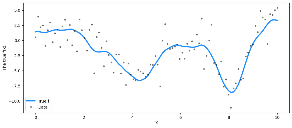
## Plot the data and the unobserved latent function
fig = plt.figure(figsize=(12, 5))
ax = fig.gca()
ax.plot(X, f_true, "dodgerblue", lw=3, label="True f")
ax.plot(X, y, "ok", ms=3, alpha=0.5, label="Data")
ax.set_xlabel("X")
ax.set_ylabel("The true f(x)")
plt.legend();

../_images/2447e8ebbc842686109ae1c94a562490c64513eb6923e57e310fd86563d08d66.png

with pm.Model() as model:
    ell = pm.Gamma("ell", alpha=2, beta=1)
    eta = pm.HalfCauchy("eta", beta=5)

    cov = eta**2 * pm.gp.cov.Matern52(1, ell)
    gp = pm.gp.Marginal(cov_func=cov)

    sigma = pm.HalfCauchy("sigma", beta=5)
    y_ = gp.marginal_likelihood("y", X=X, y=y, sigma=sigma)

    with model:
        marginal_post = pm.sample(500, tune=2000, nuts_sampler="numpyro", chains=1)

/Users/cfonnesbeck/mambaforge/envs/bayes_course/lib/python3.11/site-packages/pymc/sampling/mcmc.py:243: UserWarning: Use of external NUTS sampler is still experimental
  warnings.warn("Use of external NUTS sampler is still experimental", UserWarning)

Compiling...
Compilation time =  0:00:00.634832
Sampling...

sample: 100%|██████████| 2500/2500 [00:20<00:00, 119.94it/s, 7 steps of size 5.25e-01. acc. prob=0.92] 

Sampling time =  0:00:23.334210
Transforming variables...
Transformation time =  0:00:00.014305

summary = az.summary(marginal_post, var_names=["ell", "eta", "sigma"], round_to=2, kind="stats")
summary["True value"] = [ell_true, eta_true, sigma_true]
summary

	mean	sd	hdi_3%	hdi_97%	True value
ell	1.18	0.28	0.72	1.76	1.0
eta	4.39	1.30	2.67	7.09	3.0
sigma	1.93	0.14	1.68	2.20	2.0

The estimated values are close to their true values.

Using `.conditional`#

# new values from x=0 to x=20
X_new = np.linspace(0, 20, 600)[:, None]

# add the GP conditional to the model, given the new X values
with model:
    f_pred = gp.conditional("f_pred", X_new)

with model:
    pred_samples = pm.sample_posterior_predictive(
        marginal_post.sel(draw=slice(0, 20)), var_names=["f_pred"]
    )

Sampling: [f_pred]

100.00% [21/21 00:56<00:00]

# plot the results
fig = plt.figure(figsize=(12, 5))
ax = fig.gca()

# plot the samples from the gp posterior with samples and shading
from pymc.gp.util import plot_gp_dist

f_pred_samples = az.extract(pred_samples, group="posterior_predictive", var_names=["f_pred"])
plot_gp_dist(ax, samples=f_pred_samples.T, x=X_new)

# plot the data and the true latent function
plt.plot(X, f_true, "dodgerblue", lw=3, label="True f")
plt.plot(X, y, "ok", ms=3, alpha=0.5, label="Observed data")

# axis labels and title
plt.xlabel("X")
plt.ylim([-13, 13])
plt.title("Posterior distribution over $f(x)$ at the observed values")
plt.legend();

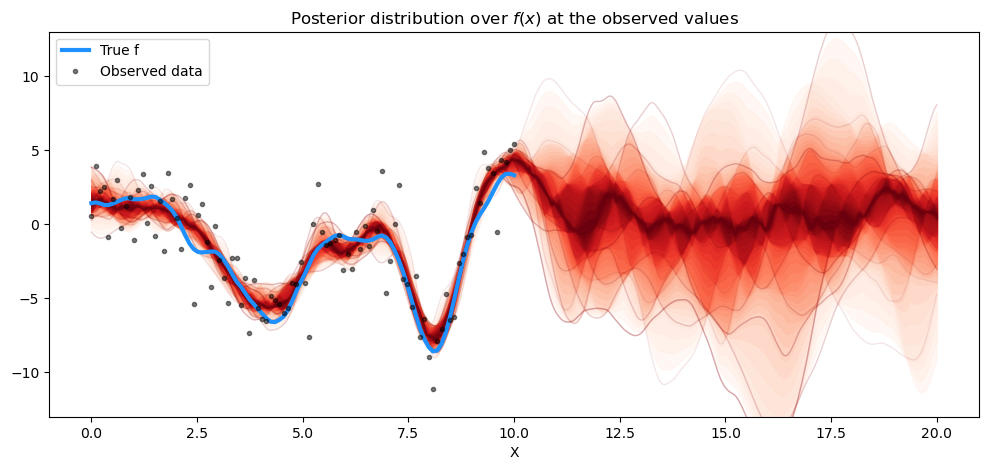
../_images/99733747e5afbc6acc61db1deecb5fe806a311fef683e5d39e6ad642ce73cc1b.png

The prediction also matches the results from gp.Latent very closely. What about predicting new data points? Here we only predicted \(f_*\), not \(f_*\) + noise, which is what we actually observe.

The conditional method of gp.Marginal contains the flag pred_noise whose default value is False. To draw from the posterior predictive distribution, we simply set this flag to True.

with model:
    y_pred = gp.conditional("y_pred", X_new, pred_noise=True)
    y_samples = pm.sample_posterior_predictive(
        marginal_post.sel(draw=slice(0, 50)), var_names=["y_pred"]
    )

Sampling: [y_pred]

100.00% [51/51 01:19<00:00]

fig = plt.figure(figsize=(12, 5))
ax = fig.gca()

# posterior predictive distribution
y_pred_samples = az.extract(y_samples, group="posterior_predictive", var_names=["y_pred"])
plot_gp_dist(ax, y_pred_samples.T, X_new, plot_samples=False, palette="bone_r")

# overlay a scatter of one draw of random points from the
#   posterior predictive distribution
plt.plot(X_new, y_pred_samples.sel(sample=1), "co", ms=2, label="Predicted data")

# plot original data and true function
plt.plot(X, y, "ok", ms=3, alpha=1.0, label="observed data")
plt.plot(X, f_true, "dodgerblue", lw=3, label="true f")

plt.xlabel("x")
plt.ylim([-13, 13])
plt.title("posterior predictive distribution, y_*")
plt.legend();

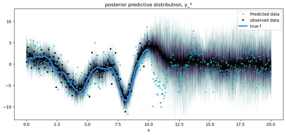
../_images/d3330db4a453e459d7141bbd2bbb73c35ad884c3a43d0f1aea92f61623917071.png

Notice that the posterior predictive density is wider than the conditional distribution of the noiseless function, and reflects the predictive distribution of the noisy data, which is marked as black dots. The light colored dots don’t follow the spread of the predictive density exactly because they are a single draw from the posterior of the GP plus noise.

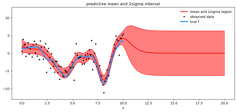
Using `.predict`#

We can use the .predict method to return the mean and variance given a particular point.

# predict
with model:
    mu, var = gp.predict(
        X_new, point=az.extract(marginal_post.posterior.sel(draw=[0])).squeeze(), diag=True
    )
sd = np.sqrt(var)

# draw plot
fig = plt.figure(figsize=(12, 5))
ax = fig.gca()

# plot mean and 2sigma intervals
plt.plot(X_new, mu, "r", lw=2, label="mean and 2σ region")
plt.plot(X_new, mu + 2 * sd, "r", lw=1)
plt.plot(X_new, mu - 2 * sd, "r", lw=1)
plt.fill_between(X_new.flatten(), mu - 2 * sd, mu + 2 * sd, color="r", alpha=0.5)

# plot original data and true function
plt.plot(X, y, "ok", ms=3, alpha=1.0, label="observed data")
plt.plot(X, f_true, "dodgerblue", lw=3, label="true f")

plt.xlabel("x")
plt.ylim([-13, 13])
plt.title("predictive mean and 2sigma interval")
plt.legend();

../_images/9d1295be5bbc6b6911dd5280f3161ded6974f82792055d55648bd4df7fea9a1e.png

Authors#

Created by Bill Engels in 2017 (pymc#1674)
Reexecuted by Colin Caroll in 2019 (pymc#3397)
Updated for V4 by Bill Engels in September 2022 (pymc-examples#237)
Updated for V5 by Chris Fonnesbeck in July 2023 (pymc-examples#549)

Watermark#

%load_ext watermark
%watermark -n -u -v -iv -w

Last updated: Mon Jun 05 2023

Python implementation: CPython
Python version       : 3.11.3
IPython version      : 8.13.2

arviz     : 0.15.1
scipy     : 1.10.1
pymc      : 5.3.0
pandas    : 2.0.2
numpy     : 1.24.3
matplotlib: 3.7.1

Watermark: 2.3.1

Categories

Tags

Marginal Likelihood Implementation#

The `.marginal_likelihood` method#

The `.conditional` distribution#

Making predictions#

Example: Regression with white, Gaussian noise#

Using `.conditional`#

Using `.predict`#

Authors#

Watermark#

Categories

Tags

Marginal Likelihood Implementation#

The .marginal_likelihood method#

The .conditional distribution#

Making predictions#

Example: Regression with white, Gaussian noise#

Using .conditional#

Using .predict#

Authors#

Watermark#

The `.marginal_likelihood` method#

The `.conditional` distribution#

Using `.conditional`#

Using `.predict`#