Using Data Containers#

import warnings

import arviz as az
import matplotlib.pyplot as plt
import numpy as np
import pandas as pd
import pymc as pm

from numpy.random import default_rng

plt.rcParams["figure.constrained_layout.use"] = True

print(f"Running on PyMC v{pm.__version__}")

Running on PyMC v5.6.0

%matplotlib inline
%config InlineBackend.figure_format = 'retina'
RANDOM_SEED = sum(map(ord, "Data Containers in PyMC"))
rng = default_rng(RANDOM_SEED)
az.style.use("arviz-darkgrid")

Introduction#

After building the statistical model of your dreams, you’re going to need to feed it some data. Data is typically introduced to a PyMC model in one of two ways. Some data is used as an exogenous input, called X in linear regression models, where mu = X @ beta. Other data are “observed” examples of the endogenous outputs of your model, called y in regression models, and is used as input to the likelihood function implied by your model. These data, either exogenous or endogenous, can be included in your model as wide variety of datatypes, including numpy ndarrays, pandas Series and DataFrame, and even pytensor TensorVariables.

Although you can pass these “raw” datatypes to your PyMC model, the best way to introduce data into your model is to use one of two pymc.Data() containers. These containers make it extremely easy to work with data in a PyMC model. They offer a range of benefits, including:

Visualization of data as a component of your probabilistic graph
Access to labeled dimensions for readability and accessibility
Support for swapping out data for out-of-sample prediction, interpolation/extrapolation, forecasting, etc.
All data will be stored in your arviz.InferenceData, which is useful for plotting and reproducible workflows.

This notebook will illustrate each of these benefits in turn, and show you the best way to integrate data into your PyMC modeling workflow.

Types of Data Containers#

PyMC offers two data containers, depending on your needs: pymc.ConstantData() and pymc.MutableData(). Both will help you visualize how data fits into your model, store the data in an InfereceData for reproducibility, and give access to labeled dimenions. As the names suggest, however, only MutableData allows you to change your data. When X is MutableData, this enables out-of-sample inference tasks. When y is MutableData, it allows you to reuse the same model on multiple datasets to perform parameter recovery studies or sensitivity analysis. These abilities do, however, come with a small performance cost.

In past versions of PyMC, the only data container was pm.Data. This container is still available for backwards compatability, but the current best practice is to use either pm.MutableData or pm.ConstantData.

Constant Data#

pm.ConstantData is a way to add fixed data to a model. It provides a speed boost in exchange for the ability to change the data. If you don’t plan on changing a given data in your model, pm.ConstantData is right for that data.

In the example shows some of the differences between using a data container, in this case pm.ConstantData, and “raw” data. This first model shows how raw data, in this case a numpy arrays, can be directly provided to a PyMC model.

true_beta = 3
true_std = 5
n_obs = 100
x = rng.normal(size=n_obs)
y = rng.normal(loc=true_beta * x, scale=true_std, size=n_obs)

with pm.Model() as no_data_model:
    beta = pm.Normal("beta")
    mu = pm.Deterministic("mu", beta * x)
    sigma = pm.Exponential("sigma", 1)
    obs = pm.Normal("obs", mu=mu, sigma=sigma, observed=y)
    idata = pm.sample(random_seed=RANDOM_SEED)

Auto-assigning NUTS sampler...
Initializing NUTS using jitter+adapt_diag...
Multiprocess sampling (4 chains in 4 jobs)
NUTS: [beta, sigma]

100.00% [8000/8000 00:00<00:00 Sampling 4 chains, 0 divergences]

Sampling 4 chains for 1_000 tune and 1_000 draw iterations (4_000 + 4_000 draws total) took 1 seconds.

Looking at the resulting computational graph, the obs node is shaded gray to indicate that it has observed data, in this case y. But the data itself is not shown on the graph, so there’s no hint about what data has been observed. In addition, the x data doesn’t appear in the graph anywhere, so it’s not obvious that this model used exogenous data as an input.

pm.model_to_graphviz(no_data_model)

../_images/ff1b9519e2ae91f4627e0a0d132657d16a25748a6598a25aaa6130240166181d.svg

Furthermore, inside idata, PyMC has automatically saved the observed (endogenous) y data, but not the exogenous x data. If we wanted to save this inference data for reuse, or to make it available as part of a reproducible research package, we would have to be sure to include the x data separately.

In this next model, we create a pm.ConstantData containers to hold the observations, and pass this container to the observed. We also make a pm.ConstantData container to hold the x data:

with pm.Model() as no_data_model:
    x_data = pm.ConstantData("x_data", x)
    y_data = pm.ConstantData("y_data", y)
    beta = pm.Normal("beta")
    mu = pm.Deterministic("mu", beta * x_data)
    sigma = pm.Exponential("sigma", 1)
    obs = pm.Normal("obs", mu=mu, sigma=sigma, observed=y_data)
    idata = pm.sample(random_seed=RANDOM_SEED)

Auto-assigning NUTS sampler...
Initializing NUTS using jitter+adapt_diag...
Multiprocess sampling (4 chains in 4 jobs)
NUTS: [beta, sigma]

100.00% [8000/8000 00:00<00:00 Sampling 4 chains, 0 divergences]

Sampling 4 chains for 1_000 tune and 1_000 draw iterations (4_000 + 4_000 draws total) took 1 seconds.

Because we used a pm.ConstantData container, the data now appears on our probabilistic graph. It is downstream from obs (since the obs variable “causes” the data), shaded in gray (because it is observed), and has a special rounded square shape to emphasize that it is data. We also see that x_data has been added to the graph.

pm.model_to_graphviz(no_data_model)

../_images/61e6b9ff445a4849a21763e3947f51f78ca20c9486f93c3feef4db8075f94a55.svg

Finally, we can check the inference data to see that the x data has been stored there as well. It is now a complete summary of all information needed to reproduce our model.

Named dimensions with data containers#

Named dimensions are another powerful benefit of working with data containers. Both pm.MutableData and pm.ConstantData allow users to keep track of dimensions (like dates or cities) and coordinates (such as the actual date times or city names) of multi-dimensional data. Both allow you to specify the dimension names and coordinates of random variables, instead of specifying the shapes of those random variables as numbers. Notice that in the previous probabilistic graphs, all of the nodes x_data, mu, obs and y_data were in a box with the number 100. A natural question for a reader to ask is, “100 what?”. Dimensions and coordinates help organize models, variables, and data by answering exactly this question.

In the next example, we generate an artifical dataset of temperatures in 3 cities over 2 months. We will then use named dimensions and coordinates to improve the readability of the model code and the quality of the visualizations.

df_data = pd.DataFrame(columns=["date"]).set_index("date")
dates = pd.date_range(start="2020-05-01", end="2020-07-01")

for city, mu in {"Berlin": 15, "San Marino": 18, "Paris": 16}.items():
    df_data[city] = rng.normal(loc=mu, size=len(dates))

df_data.index = dates
df_data.index.name = "date"
df_data.head()

	Berlin	San Marino	Paris
date
2020-05-01	15.401536	18.817801	16.836690
2020-05-02	13.575241	17.441153	14.407089
2020-05-03	14.808934	19.890369	15.616649
2020-05-04	16.071487	18.407539	15.396678
2020-05-05	15.505263	17.621143	16.723544

As noted above, ConstantData gives you the ability to give named labels to the dimensions of your data. This is done by passing a dictionary of dimension: coordinate key-value pairs to the coords argument of pymc.Model when you create your model.

For more explanation about dimensions, coordinates and their big benefits, we encourage you to take a look at the ArviZ documentation.

This is a lot of explanation – let’s see how it’s done! We will use a hierarchical model: it assumes a mean temperature for the European continent and models each city relative to the continent mean:

# The data has two dimensions: date and city
# The "coordinates" are the unique values that these dimensions can take
coords = {"date": df_data.index, "city": df_data.columns}

with pm.Model(coords=coords) as model:
    data = pm.ConstantData("observed_temp", df_data, dims=("date", "city"))

    europe_mean = pm.Normal("europe_mean_temp", mu=15.0, sigma=3.0)
    city_offset = pm.Normal("city_offset", mu=0.0, sigma=3.0, dims="city")
    city_temperature = pm.Deterministic(
        "expected_city_temp", europe_mean + city_offset, dims="city"
    )

    sigma = pm.Exponential("sigma", 1)
    pm.Normal("temperature", mu=city_temperature, sigma=sigma, observed=data, dims=("date", "city"))

    idata = pm.sample(
        random_seed=RANDOM_SEED,
    )

Auto-assigning NUTS sampler...
Initializing NUTS using jitter+adapt_diag...
Multiprocess sampling (4 chains in 4 jobs)
NUTS: [europe_mean_temp, city_offset, sigma]

100.00% [8000/8000 00:04<00:00 Sampling 4 chains, 0 divergences]

Sampling 4 chains for 1_000 tune and 1_000 draw iterations (4_000 + 4_000 draws total) took 5 seconds.

Once again, we can look at the probabilistic graph implied by our model. As before, similar node (or groups of nodes) are grouped inside plates. The plates are labeled with the dimensions of each node. Before, we had the label 100 and asked, “100 what?”. Now we see that in our model, there are 3 cities and 62 dates. Each of the 3 cities has it’s own offset, which, together with a group average, determines the estimated temperature. Finally, we see that our data is actually a 2d matrix. Adding labeled dimensions has greatly improved the presentation of our probabilistic model.

pm.model_to_graphviz(model)

../_images/75300da5d879ae4eb3626a9f4e46d3db1e501dc9635076bb58e0597ccc542ade.svg

And we see that the model did remember the coords we gave it:

for k, v in model.coords.items():
    print(f"{k}: {v[:20]}")

date: (Timestamp('2020-05-01 00:00:00'), Timestamp('2020-05-02 00:00:00'), Timestamp('2020-05-03 00:00:00'), Timestamp('2020-05-04 00:00:00'), Timestamp('2020-05-05 00:00:00'), Timestamp('2020-05-06 00:00:00'), Timestamp('2020-05-07 00:00:00'), Timestamp('2020-05-08 00:00:00'), Timestamp('2020-05-09 00:00:00'), Timestamp('2020-05-10 00:00:00'), Timestamp('2020-05-11 00:00:00'), Timestamp('2020-05-12 00:00:00'), Timestamp('2020-05-13 00:00:00'), Timestamp('2020-05-14 00:00:00'), Timestamp('2020-05-15 00:00:00'), Timestamp('2020-05-16 00:00:00'), Timestamp('2020-05-17 00:00:00'), Timestamp('2020-05-18 00:00:00'), Timestamp('2020-05-19 00:00:00'), Timestamp('2020-05-20 00:00:00'))
city: ('Berlin', 'San Marino', 'Paris')

Coordinates are automatically stored into the arviz.InferenceData object:

idata.posterior.coords

Coordinates:
  * chain    (chain) int64 0 1 2 3
  * draw     (draw) int64 0 1 2 3 4 5 6 7 8 ... 992 993 994 995 996 997 998 999
  * city     (city) <U10 'Berlin' 'San Marino' 'Paris'

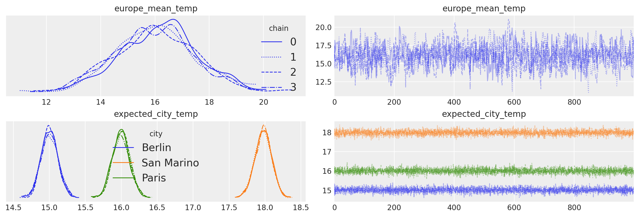
Coordinates are also used by arviz when making plots. Here we pass legend=True to az.plot_trace to automatically label the three cities in our trace plot.

axes = az.plot_trace(idata, var_names=["europe_mean_temp", "expected_city_temp"], legend=True);

../_images/28f96902e3c4fc386c4b4695bc877b44a3554a2e428c95a55aa09b85f3a78e64.png

When we use pm.ConstantData, the data are internally represented as a pytensor pytensor.tensor.TensorConstant.

type(data)

pytensor.tensor.var.TensorConstant

The values of all pytensor tensors, including both ConstantData and MutableData, can be checked using the pytensor.graph.Variable.eval() method. To access the data, we can use the pymc.Model object. All model variables, including data containers, can be accessed by indexing the model object itself with a variable name. Since this line:

    data = pm.ConstantData("observed_temp", df_data, dims=("date", "city"))

Gave the name “observed_temp” to the data, we can access it as follows:

model["observed_temp"].eval()[:15]

array([[15.40153619, 18.81780064, 16.83668986],
       [13.57524128, 17.4411525 , 14.40708945],
       [14.80893441, 19.89036942, 15.61664911],
       [16.07148689, 18.40753876, 15.39667778],
       [15.50526329, 17.62114292, 16.72354378],
       [14.86774578, 16.91297071, 16.64398094],
       [15.39861564, 18.06957647, 16.8952898 ],
       [14.82344668, 17.8925678 , 18.13033425],
       [14.29595165, 18.18139386, 14.87228836],
       [13.7296701 , 18.6225866 , 15.67262894],
       [14.68800267, 17.48605691, 15.26520975],
       [14.62891834, 19.16219466, 16.71921201],
       [14.58253668, 17.09701213, 17.10149473],
       [14.39255946, 17.66357467, 15.68899804],
       [15.8653625 , 16.66259542, 16.69857121]])

MutableData#

In many cases, you will want the ability to switch out data between model runs. This arises when you want to fit a model to multiple datasets, if you are interested in out-of-sample prediction, and in many other applications. For these cases, pm.MutableData is the correct tool.

Using MutableData container variables to fit the same model to several datasets#

We can use MutableData container variables in PyMC to fit the same model to several datasets without the need to recreate the model each time (which can be time consuming if the number of datasets is large). Note, however, that the model will still be recompilied each time.

In the next example, we will generate 10 models with a single parameter, mu. Each model will have a dataset with a different number of observations, from 10 to 100. We will use this setup to explore the effect of data quantity on parameter recovery.

# We generate 10 datasets
n_models = 10
obs_multiplier = 10

true_mu = [rng.random() for _ in range(n_models)]
observed_data = [mu + rng.normal(size=(i + 1) * obs_multiplier) for i, mu in enumerate(true_mu)]

with pm.Model() as model:
    data = pm.MutableData("data", observed_data[0])
    mu = pm.Normal("mu", 0, 10)
    pm.Normal("y", mu=mu, sigma=1, observed=data)

Once again, the name of our data is data, so we can look at it’s type. Unlike pm.ConstantData, we now see class is now pytensor.compile.sharedvalue.SharedVariable.

type(model["data"])

pytensor.tensor.sharedvar.TensorSharedVariable

This difference in type is just an implemention detail. If you are interested in learning more about the ins and outs of pytensor, you can check out this this tutorial on how Pytensor is used in PyMC. For our purposes here, we just need to know that the eval method works great for checking values:

model["data"].eval()

array([-0.10562792,  0.62102496,  1.48658991,  0.92295128,  0.43538261,
        0.73235925, -0.11983016,  0.89501808, -0.39242869,  1.4783441 ])

While eval can be used to check the values, pymc.set_data() is used to change them. Let’s use the MutableData together with pymc.set_data to repeatedly fit the same model to multiple datasets. Note that it doesn’t matter that each dataset has a different size!

# Generate one trace for each dataset
idatas = []
for data_vals in observed_data:
    with model:
        # Switch out the observed dataset
        pm.set_data({"data": data_vals})
        idatas.append(pm.sample(random_seed=RANDOM_SEED))

Show code cell output Hide code cell output

Auto-assigning NUTS sampler...
Initializing NUTS using jitter+adapt_diag...
Multiprocess sampling (4 chains in 4 jobs)
NUTS: [mu]

100.00% [8000/8000 00:00<00:00 Sampling 4 chains, 0 divergences]

Sampling 4 chains for 1_000 tune and 1_000 draw iterations (4_000 + 4_000 draws total) took 0 seconds.
Auto-assigning NUTS sampler...
Initializing NUTS using jitter+adapt_diag...
Multiprocess sampling (4 chains in 4 jobs)
NUTS: [mu]

100.00% [8000/8000 00:00<00:00 Sampling 4 chains, 0 divergences]

Sampling 4 chains for 1_000 tune and 1_000 draw iterations (4_000 + 4_000 draws total) took 0 seconds.
Auto-assigning NUTS sampler...
Initializing NUTS using jitter+adapt_diag...
Multiprocess sampling (4 chains in 4 jobs)
NUTS: [mu]

100.00% [8000/8000 00:00<00:00 Sampling 4 chains, 0 divergences]

Sampling 4 chains for 1_000 tune and 1_000 draw iterations (4_000 + 4_000 draws total) took 0 seconds.
Auto-assigning NUTS sampler...
Initializing NUTS using jitter+adapt_diag...
Multiprocess sampling (4 chains in 4 jobs)
NUTS: [mu]

100.00% [8000/8000 00:00<00:00 Sampling 4 chains, 0 divergences]

Sampling 4 chains for 1_000 tune and 1_000 draw iterations (4_000 + 4_000 draws total) took 0 seconds.
Auto-assigning NUTS sampler...
Initializing NUTS using jitter+adapt_diag...
Multiprocess sampling (4 chains in 4 jobs)
NUTS: [mu]

100.00% [8000/8000 00:00<00:00 Sampling 4 chains, 0 divergences]

Sampling 4 chains for 1_000 tune and 1_000 draw iterations (4_000 + 4_000 draws total) took 0 seconds.
Auto-assigning NUTS sampler...
Initializing NUTS using jitter+adapt_diag...
Multiprocess sampling (4 chains in 4 jobs)
NUTS: [mu]

100.00% [8000/8000 00:00<00:00 Sampling 4 chains, 0 divergences]

Sampling 4 chains for 1_000 tune and 1_000 draw iterations (4_000 + 4_000 draws total) took 0 seconds.
Auto-assigning NUTS sampler...
Initializing NUTS using jitter+adapt_diag...
Multiprocess sampling (4 chains in 4 jobs)
NUTS: [mu]

100.00% [8000/8000 00:00<00:00 Sampling 4 chains, 0 divergences]

Sampling 4 chains for 1_000 tune and 1_000 draw iterations (4_000 + 4_000 draws total) took 0 seconds.
Auto-assigning NUTS sampler...
Initializing NUTS using jitter+adapt_diag...
Multiprocess sampling (4 chains in 4 jobs)
NUTS: [mu]

100.00% [8000/8000 00:00<00:00 Sampling 4 chains, 0 divergences]

Sampling 4 chains for 1_000 tune and 1_000 draw iterations (4_000 + 4_000 draws total) took 0 seconds.
Auto-assigning NUTS sampler...
Initializing NUTS using jitter+adapt_diag...
Multiprocess sampling (4 chains in 4 jobs)
NUTS: [mu]

100.00% [8000/8000 00:00<00:00 Sampling 4 chains, 0 divergences]

Sampling 4 chains for 1_000 tune and 1_000 draw iterations (4_000 + 4_000 draws total) took 0 seconds.
Auto-assigning NUTS sampler...
Initializing NUTS using jitter+adapt_diag...
Multiprocess sampling (4 chains in 4 jobs)
NUTS: [mu]

100.00% [8000/8000 00:00<00:00 Sampling 4 chains, 0 divergences]

Sampling 4 chains for 1_000 tune and 1_000 draw iterations (4_000 + 4_000 draws total) took 0 seconds.

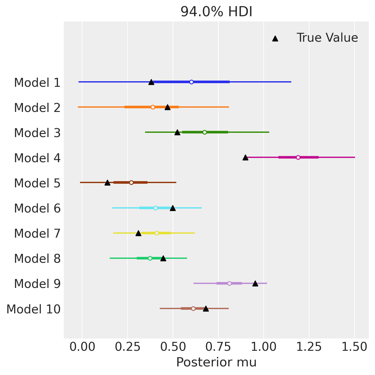
Arviz’s arviz.plot_forest() allows you to pass a list of idata objects with the same variables names. In this way, we can quickly visualize the different estimates from the 10 different datasets. We also use matplotlib to scatter the true parameter values on top of the plot_forest. We can see that as we go from 10 observations in model 1 to 100 observations in model 10, the estimates become increasing centered on the true value of mu, and the uncertainty around the estimate goes down.

model_idx = np.arange(n_models, dtype="int")
axes = az.plot_forest(idatas, var_names=["mu"], combined=True, figsize=(6, 6), legend=False)

ax = axes[0]
y_vals = np.stack([ax.get_lines()[i].get_ydata() for i in np.arange(n_models)]).ravel()
ax.scatter(true_mu, y_vals[::-1], marker="^", color="k", zorder=100, label="True Value")
ax.set(yticklabels=[f"Model {i+1}" for i in model_idx[::-1]], xlabel="Posterior mu")
ax.legend()
plt.show()

../_images/91c26f924020aa4b192bf5ff62514157151f81ec6ed5ab725cd18901297b08ed.png

Applied Example: Using MutableData as input to a binomial GLM#

A common task in machine learning is to predict values for unseen data, and the MutableData container variable is exactly what we need to do this.

One small detail to pay attention to in this case is that the shapes of the input data (x) and output data (obs) must be the same. When we make out-of-sample predictions, we typically change only the input data, the shape of which may not be the same as the training observations. Naively changing only one will result in a shape error. There are two solutions:

Use a pm.MutableData for the x data and the y data, and use pm.set_data to change y to something of the same shape as the test inputs.
Tell PyMC that the shape of the obs should always be the shape of the input data.

In the next model, we use option 2. This way, we don’t need to pass dummy data to y every time we want to change x.

n_obs = 100
true_beta = 1.5
true_alpha = 0.25

x = rng.normal(size=n_obs)
true_p = 1 / (1 + np.exp(-(true_alpha + true_beta * x)))
y = rng.binomial(n=1, p=true_p)

As you can see, we can even mix-and-match pm.ConstantData and pm.MutableData, depending on which data we plan to change. In this example, we don’t plan to do any post-estimation tasks with y, so we can put it in a ConstantData container.

with pm.Model() as logistic_model:
    x_data = pm.MutableData("x", x)
    y_data = pm.ConstantData("y", y)

    alpha = pm.Normal("alpha")
    beta = pm.Normal("beta")

    p = pm.Deterministic("p", pm.math.sigmoid(alpha + beta * x_data))

    # Here is were we link the shapes of the inputs (x_data) and the observed varaiable
    # It will be the shape we tell it, rather than the (constant!) shape of y_data
    obs = pm.Bernoulli("obs", p=p, observed=y_data, shape=x_data.shape[0])

    # fit the model
    idata = pm.sample(random_seed=RANDOM_SEED)

    # Generate a counterfactual dataset using our model
    idata = pm.sample_posterior_predictive(
        idata, extend_inferencedata=True, random_seed=RANDOM_SEED
    )

Auto-assigning NUTS sampler...
Initializing NUTS using jitter+adapt_diag...
Multiprocess sampling (4 chains in 4 jobs)
NUTS: [alpha, beta]

100.00% [8000/8000 00:00<00:00 Sampling 4 chains, 0 divergences]

Sampling 4 chains for 1_000 tune and 1_000 draw iterations (4_000 + 4_000 draws total) took 1 seconds.
Sampling: [obs]

100.00% [4000/4000 00:00<00:00]

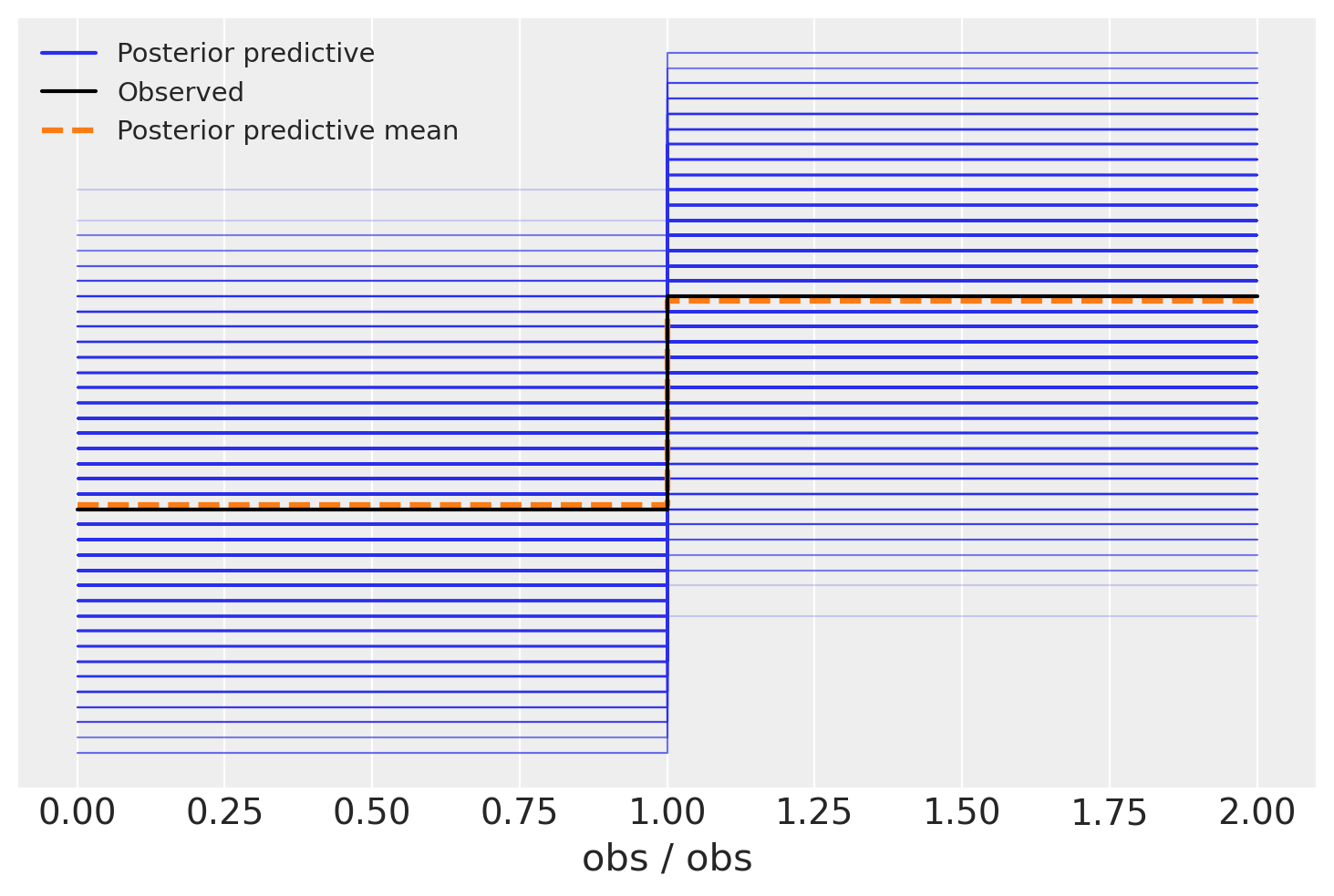
A common post-estimation diagonstic is to look at a posterior predictive plot, using arviz.plot_ppc(). This shows the distribution of data sampled from your model along side the observed data. If they look similar, we have some evidence that the model isn’t so bad.

In this case, however, it can be difficult to interpret a posterior predictive plot. Since we’re doing a logistic regression, observed values can only be zero or one. As a result, the posterior predictive graph has this tetris-block shape. What are we to make of it? Evidently our model produces more 1’s than 0’s, and the mean proportion matches the data. But there’s also a lot of uncertainty in that proportion. We else can we say about the model’s performance?

az.plot_ppc(idata)

<Axes: xlabel='obs / obs'>

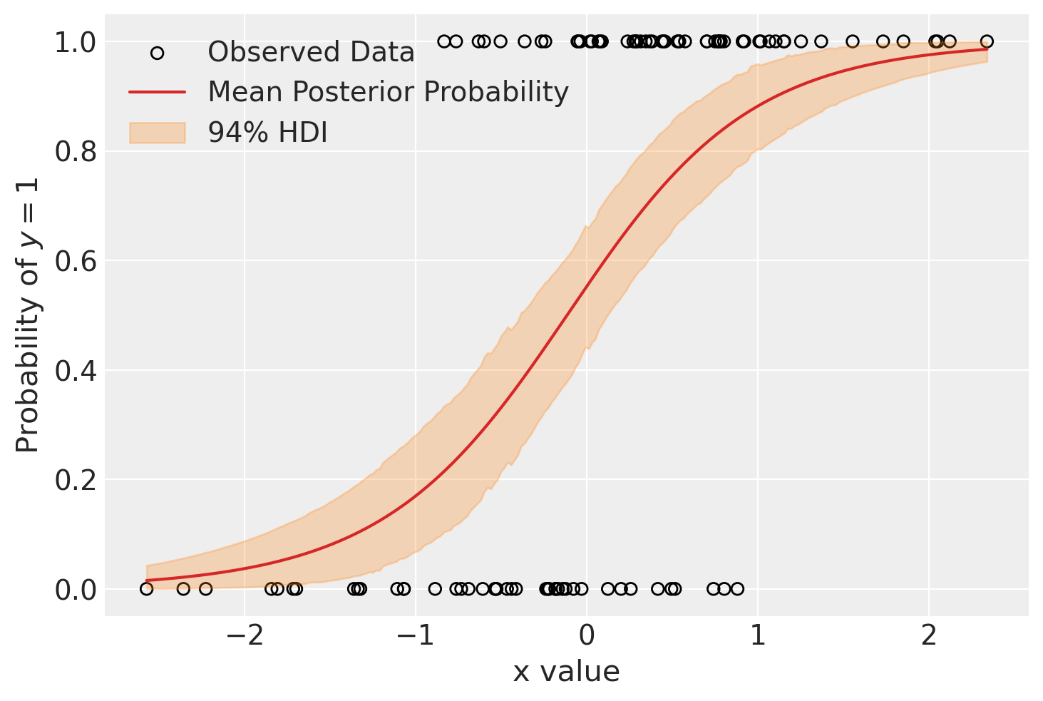
../_images/280ff47bb38f12fc478ffc31b69ee2616fea24b56a5e996c36a75f0be7302418.png

Another graph we could make to see how our model is doing is to look at how the latent variable p evolves over the space of covariates. We expect some relationship between the covariate and the data, and our model encodes that relationship in the variable p. In this model, the only covariate is x. If the relationship between x and y is positive, we expect low p and lots of observed zeros where x is small, and high p and lots of observed ones where it is large.

That’s nice and all, but for plotting x is all jumbled up. Admittedly, we could just sort the values. But another way (that shows off how to use our MutableData!) is to pass an evenly spaced grid of x values into our model. This corresponds to making a preditiction for p at every point on the grid, which will give us a nice plottable result. This is also how we could do interpolation of extrapolation using our model, so it’s a very nice technique to know.

In the next code block, we swap out the (randomly shuffled) values of x for an evenly-spaced grid of values that spans the range of observed x.

grid_size = 250
x_grid = np.linspace(x.min(), x.max(), grid_size)
with logistic_model:
    # Switch out the observations and use `sample_posterior_predictive` to predict
    # We do not need to set data for the outputs because we told the model to always link the shape of the output to the shape
    # of the input.
    pm.set_data({"x": x_grid})
    post_idata = pm.sample_posterior_predictive(
        idata, var_names=["p", "obs"], random_seed=RANDOM_SEED
    )

Sampling: [obs]

100.00% [4000/4000 00:00<00:00]

Using the new post_idata, which holds the out-of-sample “predictions” for p, we make the plot of x_grid against p. We also plot the observed data. We can see that the model expects low probability (p) where x is small, and that the probability changes very gradually with x.

fig, ax = plt.subplots()
hdi = az.hdi(post_idata.posterior_predictive.p).p

ax.scatter(x, y, facecolor="none", edgecolor="k", label="Observed Data")
p_mean = post_idata.posterior_predictive.p.mean(dim=["chain", "draw"])
ax.plot(x_grid, p_mean, color="tab:red", label="Mean Posterior Probability")
ax.fill_between(x_grid, *hdi.values.T, color="tab:orange", alpha=0.25, label="94% HDI")
ax.legend()
ax.set(ylabel="Probability of $y=1$", xlabel="x value")
plt.show()

../_images/0ae54bf59221ef075fed306415c2dbb3756598028d937974141da2aa02cf5389.png

The same concept applied to a more complex model can be seen in the notebook Variational Inference: Bayesian Neural Networks.

Applied example: height of toddlers as a function of age#

This example is taken from Osvaldo Martin’s book: Bayesian Analysis with Python: Introduction to statistical modeling and probabilistic programming using PyMC and ArviZ, 2nd Edition [Martin, 2018].

The World Health Organization and other health institutions around the world collect data for newborns and toddlers and design growth charts standards. These charts are an essential component of the paediatric toolkit and also as a measure of the general well-being of populations in order to formulate health policies, and plan interventions and monitor their effectiveness.

An example of such data is the lengths (heights) of newborn / toddler girls as a function of age (in months):

try:
    data = pd.read_csv("../data/babies.csv")
except FileNotFoundError:
    data = pd.read_csv(pm.get_data("babies.csv"))
data.plot.scatter("Month", "Length", alpha=0.4);

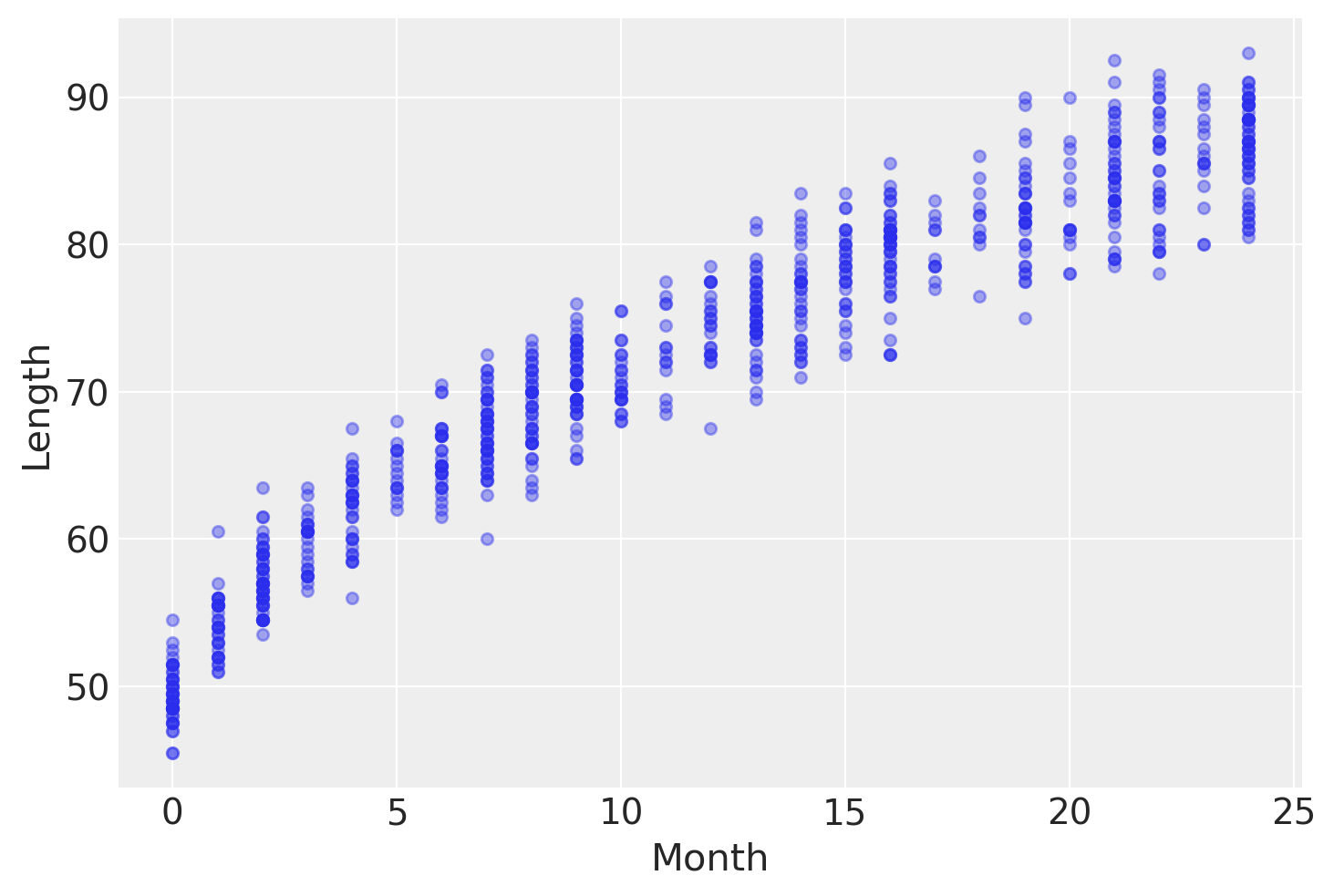
../_images/a4c3ca0e16d44479e8212733340e261c450aa712af1af0ac260c49a3a098cb92.png

To model this data, we will introduce one new feature: mutable coords. When we know we have a coord that is going to need to change in the future, like the index of data we will change between training and test sets, we can set the model coords via the coords_mutable keyword argument.

You are also allowed to specify both coords and coords_mutable in the same model. In this next model, we will always have the same parameters, so the parameters coord is specified as constant via coords, while the obs_idx will change when we go to do out-of-sample prediction.

Finally, we plan to use to use this model to do some out-of-sample prediction. Thus, we will opt for pm.MutableData as the data container. Note that we are allowed to label the dimensions of a pm.MutableData just like pm.ConstantData.

with pm.Model(
    coords_mutable={"obs_idx": np.arange(len(data))}, coords={"parameter": ["intercept", "slope"]}
) as model_babies:
    mean_params = pm.Normal("mean_params", sigma=10, dims=["parameter"])
    sigma_params = pm.Normal("sigma_params", sigma=10, dims=["parameter"])
    month = pm.MutableData("month", data.Month.values.astype(float), dims=["obs_idx"])

    mu = pm.Deterministic("mu", mean_params[0] + mean_params[1] * month**0.5, dims=["obs_idx"])
    sigma = pm.Deterministic("sigma", sigma_params[0] + sigma_params[1] * month, dims=["obs_idx"])

    length = pm.Normal("length", mu=mu, sigma=sigma, observed=data.Length, dims=["obs_idx"])

    idata_babies = pm.sample(random_seed=RANDOM_SEED)

Auto-assigning NUTS sampler...
Initializing NUTS using jitter+adapt_diag...
Multiprocess sampling (4 chains in 4 jobs)
NUTS: [mean_params, sigma_params]

100.00% [8000/8000 00:01<00:00 Sampling 4 chains, 0 divergences]

Sampling 4 chains for 1_000 tune and 1_000 draw iterations (4_000 + 4_000 draws total) took 2 seconds.

The following figure shows the result of our model. The expected length, \(\mu\), is represented with a blue curve, and two semi-transparent orange bands represent the 60% and 94% highest posterior density intervals of posterior predictive length measurements:

with model_babies:
    pm.sample_posterior_predictive(idata_babies, extend_inferencedata=True, random_seed=RANDOM_SEED)

Sampling: [length]

100.00% [4000/4000 00:00<00:00]

ax = az.plot_hdi(
    data.Month,
    idata_babies.posterior_predictive["length"],
    hdi_prob=0.6,
    fill_kwargs={"alpha": 0.8},
)
ax.plot(
    data.Month,
    idata_babies.posterior["mu"].mean(("chain", "draw")),
    label="Posterior predictive mean",
)
ax = az.plot_lm(
    idata=idata_babies,
    y="length",
    x="month",
    kind_pp="hdi",
    y_kwargs={"color": "k", "ms": 6, "alpha": 0.15},
    y_hat_fill_kwargs=dict(fill_kwargs={"alpha": 0.4}),
    axes=ax,
)

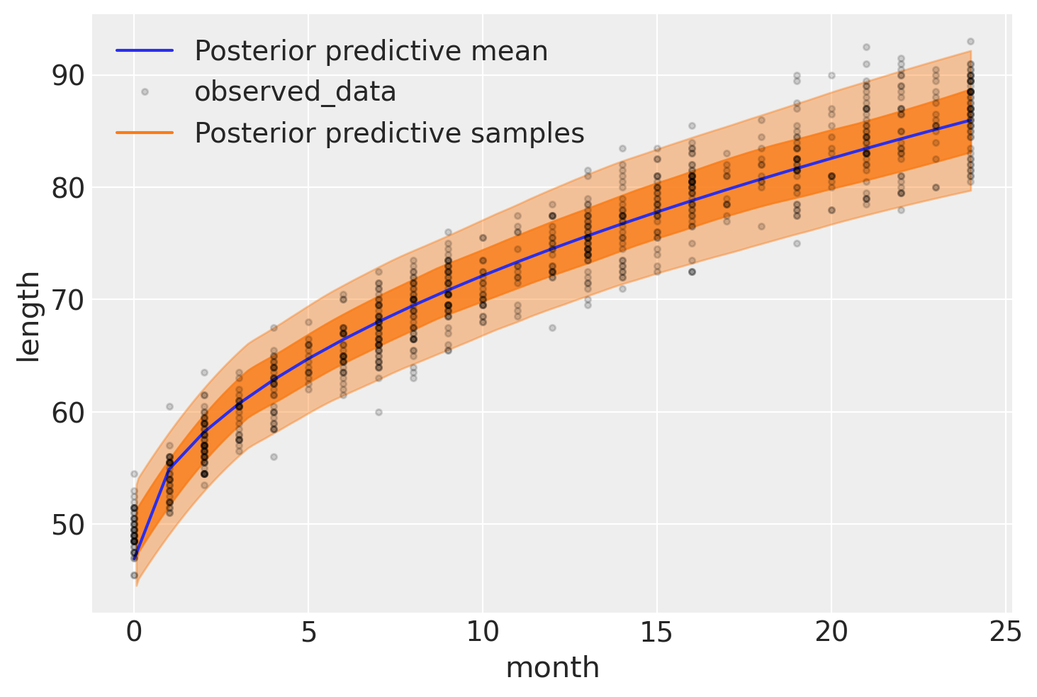
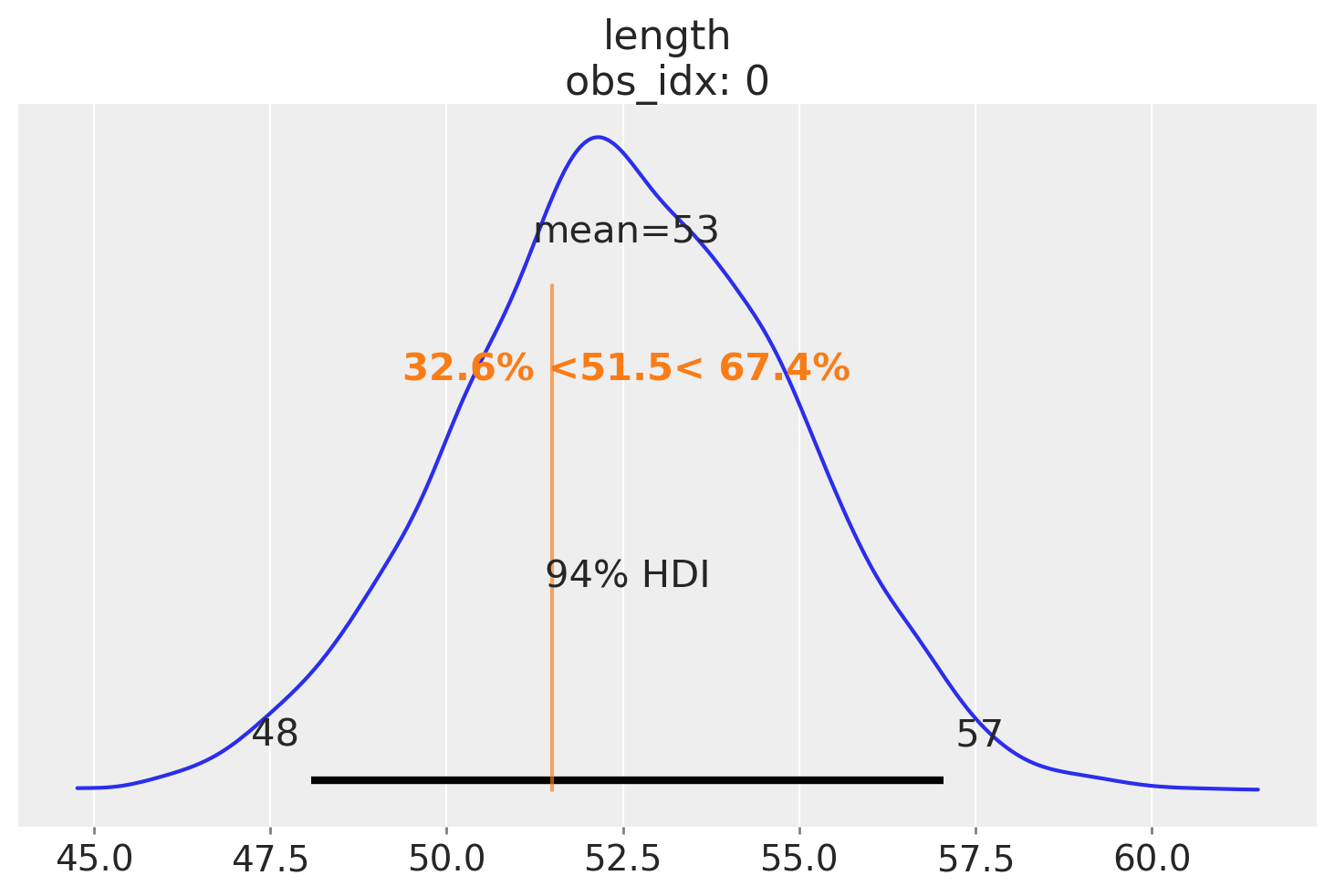
../_images/bad25ced6620ec3c88961f26d4a1b696cafb176c33fc122dc3f44f6274a2e379.png

At the moment of writing Osvaldo’s daughter is two weeks (\(\approx 0.5\) months) old, and thus he wonders how her length compares to the growth chart we have just created. One way to answer this question is to ask the model for the distribution of the variable length for babies of 0.5 months. Using PyMC we can ask this questions with the function sample_posterior_predictive , as this will return samples of Length conditioned on the obseved data and the estimated distribution of parameters, that is including uncertainties.

The only problem is that by default this function will return predictions for Length for the observed values of Month, and \(0.5\) months (the value Osvaldo cares about) has not been observed, – all measures are reported for integer months. The easier way to get predictions for non-observed values of Month is to pass new values to the Data container we defined above in our model. To do that, we need to use pm.set_data and then we just have to sample from the posterior predictve distribution. We will also have to set coords for these new observations, which we are allowed to do in the pm.set_data function because we have set the obs_idx coord as mutable.

Note that the actual value we pass for obs_idx is totally irrevelant in this case, so we give it a value of 0. What is important is that we update it to have the same length as the ages we want to do out-of-sample prediction for, and that each age has a unique index identifier.

ages_to_check = [0.5]
with model_babies:
    pm.set_data({"month": ages_to_check}, coords={"obs_idx": [0]})

    # Setting predictions=True will add a new "predictions" group to our idata. This lets us store the posterior,
    # posterior_predictive, and predictions all in the same object.
    idata_babies = pm.sample_posterior_predictive(
        idata_babies, extend_inferencedata=True, predictions=True, random_seed=RANDOM_SEED
    )

Sampling: [length]

100.00% [4000/4000 00:00<00:00]

Now we can plot the expected distribution of lengths for 2-week old babies and compute additional quantities – for example the percentile of a child given her length. Here, let’s imagine that the child we’re interested in has a length of 51.5:

ref_length = 51.5

az.plot_posterior(
    idata_babies,
    group="predictions",
    ref_val={"length": [{"ref_val": ref_length}]},
    labeller=az.labels.DimCoordLabeller(),
);

../_images/22729a24f6e02df321c6b723a073a6d9c24c76eeef5d5e7d36859f324ccd29e7.png

Authors#

Authored by Juan Martin Loyola in March, 2019 (pymc#3389)
Updated by Kavya Jaiswal and Oriol Abril in December, 2021 (pymc-examples#151)
Updated by Jesse Grabowski in July 2023 (pymc-examples#559)

References#

[1]

Osvaldo Martin. Bayesian analysis with Python: introduction to statistical modeling and probabilistic programming using PyMC3 and ArviZ. Packt Publishing Ltd, 2018.

Watermark#

%load_ext watermark
%watermark -n -u -v -iv -w -p pytensor,xarray

Last updated: Sat Jul 15 2023

Python implementation: CPython
Python version       : 3.10.12
IPython version      : 8.14.0

pytensor: 2.12.3
xarray  : 2023.6.0

pymc      : 5.6.0
matplotlib: 3.7.2
pandas    : 2.0.3
arviz     : 0.15.1
numpy     : 1.24.4

Watermark: 2.4.3

License notice#

All the notebooks in this example gallery are provided under the MIT License which allows modification, and redistribution for any use provided the copyright and license notices are preserved.

Citing PyMC examples#

To cite this notebook, use the DOI provided by Zenodo for the pymc-examples repository.

Important

Many notebooks are adapted from other sources: blogs, books… In such cases you should cite the original source as well.

Also remember to cite the relevant libraries used by your code.

Here is an citation template in bibtex:

@incollection{citekey,
  author    = "<notebook authors, see above>",
  title     = "<notebook title>",
  editor    = "PyMC Team",
  booktitle = "PyMC examples",
  doi       = "10.5281/zenodo.5654871"
}

which once rendered could look like:

Categories

Tags

Using Data Containers#

Introduction#

Types of Data Containers#

Constant Data#

Named dimensions with data containers#

MutableData#

Using MutableData container variables to fit the same model to several datasets#

Applied Example: Using MutableData as input to a binomial GLM#

Applied example: height of toddlers as a function of age#

Authors#

References#

Watermark#

License notice#

Citing PyMC examples#