Model Averaging#
import arviz as az
import matplotlib.pyplot as plt
import numpy as np
import pandas as pd
import pymc3 as pm

print(f"Running on PyMC3 v{pm.__version__}")
Running on PyMC3 v3.11.5
RANDOM_SEED = 8927
np.random.seed(RANDOM_SEED)
az.style.use("arviz-darkgrid")
When confronted with more than one model we have several options. One of them is to perform model selection, using for example a given Information Criterion as exemplified the PyMC examples Model comparison and the GLM: Model Selection. Model selection is appealing for its simplicity, but we are discarding information about the uncertainty in our models. This is somehow similar to computing the full posterior and then just keep a point-estimate like the posterior mean; we may become overconfident of what we really know. You can also browse the blog/tag/model-comparison tag to find related posts.
One alternative is to perform model selection but discuss all the different models together with the computed values of a given Information Criterion. It is important to put all these numbers and tests in the context of our problem so that we and our audience can have a better feeling of the possible limitations and shortcomings of our methods. If you are in the academic world you can use this approach to add elements to the discussion section of a paper, presentation, thesis, and so on.
Yet another approach is to perform model averaging. The idea now is to generate a meta-model (and meta-predictions) using a weighted average of the models. There are several ways to do this and PyMC includes 3 of them that we are going to briefly discuss, you will find a more thorough explanation in the work by Yao et al. [2018]. PyMC integrates with ArviZ for model comparison.
Pseudo Bayesian model averaging#
Bayesian models can be weighted by their marginal likelihood, this is known as Bayesian Model Averaging. While this is theoretically appealing, it is problematic in practice: on the one hand the marginal likelihood is highly sensible to the specification of the prior, in a way that parameter estimation is not, and on the other, computing the marginal likelihood is usually a challenging task. An alternative route is to use the values of WAIC (Widely Applicable Information Criterion) or LOO (pareto-smoothed importance sampling Leave-One-Out cross-validation), which we will call generically IC, to estimate weights. We can do this by using the following formula:
Where \(dIC_i\) is the difference between the i-esim information criterion value and the lowest one. Remember that the lowest the value of the IC, the better. We can use any information criterion we want to compute a set of weights, but, of course, we cannot mix them.
This approach is called pseudo Bayesian model averaging, or Akaike-like weighting and is an heuristic way to compute the relative probability of each model (given a fixed set of models) from the information criteria values. Look how the denominator is just a normalization term to ensure that the weights sum up to one.
Pseudo Bayesian model averaging with Bayesian Bootstrapping#
The above formula for computing weights is a very nice and simple approach, but with one major caveat it does not take into account the uncertainty in the computation of the IC. We could compute the standard error of the IC (assuming a Gaussian approximation) and modify the above formula accordingly. Or we can do something more robust, like using a Bayesian Bootstrapping to estimate, and incorporate this uncertainty.
Stacking#
The third approach implemented in PyMC is known as stacking of predictive distributions by Yao et al. [2018]. We want to combine several models in a metamodel in order to minimize the divergence between the meta-model and the true generating model, when using a logarithmic scoring rule this is equivalent to:
Where \(n\) is the number of data points and \(K\) the number of models. To enforce a solution we constrain \(w\) to be \(w_k \ge 0\) and \(\sum_{k=1}^{K} w_k = 1\).
The quantity \(p(y_i|y_{-i}, M_k)\) is the leave-one-out predictive distribution for the \(M_k\) model. Computing it requires fitting each model \(n\) times, each time leaving out one data point. Fortunately we can approximate the exact leave-one-out predictive distribution using LOO (or even WAIC), and that is what we do in practice.
Weighted posterior predictive samples#
Once we have computed the weights, using any of the above 3 methods, we can use them to get a weighted posterior predictive samples. PyMC offers functions to perform these steps in a simple way, so let see them in action using an example.
The following example is taken from the superb book McElreath [2018] by Richard McElreath. You will find more PyMC examples from this book in the repository Statistical-Rethinking-with-Python-and-PyMC. We are going to explore a simplified version of it. Check the book for the whole example and a more thorough discussion of both, the biological motivation for this problem and a theoretical/practical discussion of using Information Criteria to compare, select and average models.
Briefly, our problem is as follows: We want to explore the composition of milk across several primate species, it is hypothesized that females from species of primates with larger brains produce more nutritious milk (loosely speaking this is done in order to support the development of such big brains). This is an important question for evolutionary biologists and try to give an answer we will use 3 variables, two predictor variables: the proportion of neocortex compare to the total mass of the brain and the logarithm of the body mass of the mothers. And for predicted variable, the kilocalories per gram of milk. With these variables we are going to build 3 different linear models:
A model using only the neocortex variable
A model using only the logarithm of the mass variable
A model using both variables
Let start by uploading the data and centering the neocortex and log mass variables, for better sampling.
d = pd.read_csv(
    "https://raw.githubusercontent.com/pymc-devs/resources/master/Rethinking_2/Data/milk.csv",
    sep=";",
)
d = d[["kcal.per.g", "neocortex.perc", "mass"]].rename({"neocortex.perc": "neocortex"}, axis=1)
d["log_mass"] = np.log(d["mass"])
d = d[~d.isna().any(axis=1)].drop("mass", axis=1)
d.iloc[:, 1:] = d.iloc[:, 1:] - d.iloc[:, 1:].mean()
d.head()
| kcal.per.g | neocortex | log_mass | |
|---|---|---|---|
| 0 | 0.49 | -12.415882 | -0.831486 |
| 5 | 0.47 | -3.035882 | 0.158913 |
| 6 | 0.56 | -3.035882 | 0.181513 |
| 7 | 0.89 | 0.064118 | -0.579032 |
| 9 | 0.92 | 1.274118 | -1.884978 |
Now that we have the data we are going to build our first model using only the neocortex.
with pm.Model() as model_0:
    alpha = pm.Normal("alpha", mu=0, sigma=10)
    beta = pm.Normal("beta", mu=0, sigma=10)
    sigma = pm.HalfNormal("sigma", 10)

    mu = alpha + beta * d["neocortex"]

    kcal = pm.Normal("kcal", mu=mu, sigma=sigma, observed=d["kcal.per.g"])
    trace_0 = pm.sample(2000, return_inferencedata=True)
Auto-assigning NUTS sampler...
Initializing NUTS using jitter+adapt_diag...
Multiprocess sampling (2 chains in 2 jobs)
NUTS: [sigma, beta, alpha]
Sampling 2 chains for 1_000 tune and 2_000 draw iterations (2_000 + 4_000 draws total) took 12 seconds.
The second model is exactly the same as the first one, except we now use the logarithm of the mass
with pm.Model() as model_1:
    alpha = pm.Normal("alpha", mu=0, sigma=10)
    beta = pm.Normal("beta", mu=0, sigma=1)
    sigma = pm.HalfNormal("sigma", 10)

    mu = alpha + beta * d["log_mass"]

    kcal = pm.Normal("kcal", mu=mu, sigma=sigma, observed=d["kcal.per.g"])

    trace_1 = pm.sample(2000, return_inferencedata=True)
Auto-assigning NUTS sampler...
Initializing NUTS using jitter+adapt_diag...
Multiprocess sampling (2 chains in 2 jobs)
NUTS: [sigma, beta, alpha]
Sampling 2 chains for 1_000 tune and 2_000 draw iterations (2_000 + 4_000 draws total) took 11 seconds.
The acceptance probability does not match the target. It is 0.8826043398520717, but should be close to 0.8. Try to increase the number of tuning steps.
And finally the third model using the neocortex and log_mass variables
with pm.Model() as model_2:
    alpha = pm.Normal("alpha", mu=0, sigma=10)
    beta = pm.Normal("beta", mu=0, sigma=1, shape=2)
    sigma = pm.HalfNormal("sigma", 10)

    mu = alpha + pm.math.dot(beta, d[["neocortex", "log_mass"]].T)

    kcal = pm.Normal("kcal", mu=mu, sigma=sigma, observed=d["kcal.per.g"])

    trace_2 = pm.sample(2000, return_inferencedata=True)
Auto-assigning NUTS sampler...
Initializing NUTS using jitter+adapt_diag...
Multiprocess sampling (2 chains in 2 jobs)
NUTS: [sigma, beta, alpha]
Sampling 2 chains for 1_000 tune and 2_000 draw iterations (2_000 + 4_000 draws total) took 12 seconds.
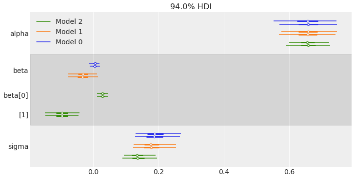
Now that we have sampled the posterior for the 3 models, we are going to compare them visually. One option is to use the forestplot function that supports plotting more than one trace.
traces = [trace_0, trace_1, trace_2]
az.plot_forest(traces, figsize=(10, 5));

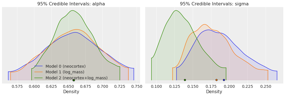
Another option is to plot several traces in a same plot is to use plot_density. This plot is somehow similar to a forestplot, but we get truncated KDE (kernel density estimation) plots (by default 95% credible intervals) grouped by variable names together with a point estimate (by default the mean).
ax = az.plot_density(
    traces,
    var_names=["alpha", "sigma"],
    shade=0.1,
    data_labels=["Model 0 (neocortex)", "Model 1 (log_mass)", "Model 2 (neocortex+log_mass)"],
)

ax[0, 0].set_xlabel("Density")
ax[0, 0].set_ylabel("")
ax[0, 0].set_title("95% Credible Intervals: alpha")

ax[0, 1].set_xlabel("Density")
ax[0, 1].set_ylabel("")
ax[0, 1].set_title("95% Credible Intervals: sigma")
Text(0.5, 1.0, '95% Credible Intervals: sigma')

Now that we have sampled the posterior for the 3 models, we are going to use WAIC (Widely applicable information criterion) to compare the 3 models. We can do this using the compare function included with ArviZ.
model_dict = dict(zip(["model_0", "model_1", "model_2"], traces))
comp = az.compare(model_dict)
comp
| rank | loo | p_loo | d_loo | weight | se | dse | warning | loo_scale | |
|---|---|---|---|---|---|---|---|---|---|
| model_2 | 0 | 8.365702 | 3.159733 | 0.000000 | 1.000000e+00 | 2.523747 | 0.000000 | False | log |
| model_1 | 1 | 4.485976 | 2.017674 | 3.879726 | 5.162537e-15 | 2.054953 | 1.705681 | False | log |
| model_0 | 2 | 3.419154 | 2.078996 | 4.946548 | 0.000000e+00 | 1.577262 | 2.453546 | False | log |
We can see that the best model is model_2, the one with both predictor variables. Notice the DataFrame is ordered from lowest to highest WAIC (i.e from better to worst model). Check the Model comparison for a more detailed discussion on model comparison.
We can also see that we get a column with the relative weight for each model (according to the first equation at the beginning of this notebook). This weights can be vaguely interpreted as the probability that each model will make the correct predictions on future data. Of course this interpretation is conditional on the models used to compute the weights, if we add or remove models the weights will change. And also is dependent on the assumptions behind WAIC (or any other Information Criterion used). So try to not overinterpret these weights.
Now we are going to use computed weights to generate predictions based not on a single model, but on the weighted set of models. This is one way to perform model averaging. Using PyMC we can call the sample_posterior_predictive_w function as follows:
ppc_w = pm.sample_posterior_predictive_w(
    traces=traces,
    models=[model_0, model_1, model_2],
    weights=comp.weight.sort_index(ascending=True),
    progressbar=True,
)
Notice that we are passing the weights ordered by their index. We are doing this because we pass traces and models ordered from model 0 to 2, but the computed weights are ordered from lowest to highest WAIC (or equivalently from larger to lowest weight). In summary, we must be sure that we are correctly pairing the weights and models.
We are also going to compute PPCs for the lowest-WAIC model.
ppc_2 = pm.sample_posterior_predictive(trace=trace_2, model=model_2, progressbar=False)
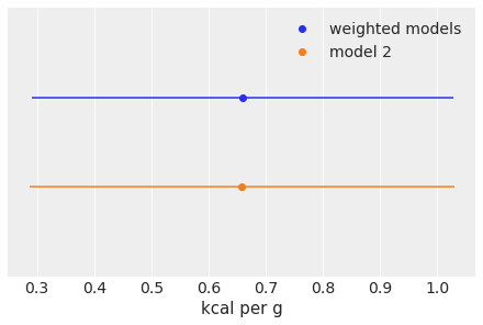
A simple way to compare both kind of predictions is to plot their mean and hpd interval.
mean_w = ppc_w["kcal"].mean()
hpd_w = az.hdi(ppc_w["kcal"].flatten())

mean = ppc_2["kcal"].mean()
hpd = az.hdi(ppc_2["kcal"].flatten())

plt.plot(mean_w, 1, "C0o", label="weighted models")
plt.hlines(1, *hpd_w, "C0")
plt.plot(mean, 0, "C1o", label="model 2")
plt.hlines(0, *hpd, "C1")

plt.yticks([])
plt.ylim(-1, 2)
plt.xlabel("kcal per g")
plt.legend();

As we can see the mean value is almost the same for both predictions but the uncertainty in the weighted model is larger. We have effectively propagated the uncertainty about which model we should select to the posterior predictive samples. You can now try with the other two methods for computing weights stacking (the default and recommended method) and pseudo-BMA.
Final notes:
There are other ways to average models such as, for example, explicitly building a meta-model that includes all the models we have. We then perform parameter inference while jumping between the models. One problem with this approach is that jumping between models could hamper the proper sampling of the posterior.
Besides averaging discrete models we can sometimes think of continuous versions of them. A toy example is to imagine that we have a coin and we want to estimated its degree of bias, a number between 0 and 1 having a 0.5 equal chance of head and tails (fair coin). We could think of two separate models one with a prior biased towards heads and one towards tails. We could fit both separate models and then average them using, for example, IC-derived weights. An alternative, is to build a hierarchical model to estimate the prior distribution, instead of contemplating two discrete models we will be computing a continuous model that includes these the discrete ones as particular cases. Which approach is better? That depends on our concrete problem. Do we have good reasons to think about two discrete models, or is our problem better represented with a continuous bigger model?
References#
Richard McElreath. Statistical rethinking: A Bayesian course with examples in R and Stan. Chapman and Hall/CRC, 2018.
Yuling Yao, Aki Vehtari, Daniel Simpson, and Andrew Gelman. Using stacking to average bayesian predictive distributions (with discussion). Bayesian Analysis, sep 2018. URL: https://doi.org/10.1214\%2F17-ba1091, doi:10.1214/17-ba1091.
Watermark#
%load_ext watermark
%watermark -n -u -v -iv -w
Last updated: Sun Aug 21 2022

Python implementation: CPython
Python version       : 3.10.5
IPython version      : 8.4.0

pandas    : 1.4.3
matplotlib: 3.5.2
numpy     : 1.22.1
arviz     : 0.12.1
pymc3     : 3.11.5

Watermark: 2.3.1
License notice#
All the notebooks in this example gallery are provided under the MIT License which allows modification, and redistribution for any use provided the copyright and license notices are preserved.
Citing PyMC examples#
To cite this notebook, use the DOI provided by Zenodo for the pymc-examples repository.
Important
Many notebooks are adapted from other sources: blogs, books… In such cases you should cite the original source as well.
Also remember to cite the relevant libraries used by your code.
Here is an citation template in bibtex:
@incollection{citekey,
  author    = "<notebook authors, see above>",
  title     = "<notebook title>",
  editor    = "PyMC Team",
  booktitle = "PyMC examples",
  doi       = "10.5281/zenodo.5654871"
}
which once rendered could look like: