Reliability Statistics and Predictive Calibration#
Attention
This notebook uses libraries that are not PyMC dependencies and therefore need to be installed specifically to run this notebook. Open the dropdown below for extra guidance.
Extra dependencies install instructions
In order to run this notebook (either locally or on binder) you won’t only need a working PyMC installation with all optional dependencies, but also to install some extra dependencies. For advise on installing PyMC itself, please refer to Installation
You can install these dependencies with your preferred package manager, we provide as an example the pip and conda commands below.
$ pip install lifelines
Note that if you want (or need) to install the packages from inside the notebook instead of the command line, you can install the packages by running a variation of the pip command:
import sys
!{sys.executable} -m pip install lifelines
You should not run !pip install as it might install the package in a different
environment and not be available from the Jupyter notebook even if installed.
Another alternative is using conda instead:
$ conda install lifelines
when installing scientific python packages with conda, we recommend using conda forge
import os
import random

from io import StringIO

import arviz as az
import matplotlib.cm as cm
import matplotlib.pyplot as plt
import numpy as np
import pandas as pd
import pymc as pm

from lifelines import KaplanMeierFitter, LogNormalFitter, WeibullFitter
from lifelines.utils import survival_table_from_events
from scipy.stats import binom, lognorm, norm, weibull_min
RANDOM_SEED = 8927
rng = np.random.default_rng(RANDOM_SEED)
az.style.use("arviz-darkgrid")
%config InlineBackend.figure_format = 'retina'
Reliability Statistics#
When we want to make inferences about likely failures on a production line, we may have large or small sample data set depending on the industry, nature of the goods or specificifty of the question we’re seeking to answer. But in all cases there is a question of cost and a quantity of tolerable failures.
A reliability study therefore has to account for the period in which a failure is important to observe, the cost of the failure and cost of running a mis-specified study. The requirements for precision in the definition of the question and the nature of the modelling exercise are paramount.
The key feature of time-to-failure data is the manner in which it is censored and how this biases traditional statistical summaries and estimation techniques. In this notebook we’re going to focus on the prediction of failure times and compare the Bayesian notion of a calibrated prediction interval to some frequentist alternatives. We draw on the work in the book Statistical Methods for Reliability Data. For details (see Meeker et al. [2022])
Types of Prediction#
We might want to know about different views of the failure time distribution such as:
Time to failure of a new item
Time until k failures in a future sample of m units
While there are non-parametric and descriptive methods that can be used to assess these kinds of question we’re going to focus on the case where we have a probability model e.g. a lognormal distribution of failure times \(F(t: \mathbf{\theta})\) parameterised by an unknown \(\mathbf{\theta}\).
Structure of the Presentation#
We will
Discuss non-parametric estimates of the cumulative density function CDF for reliability data
Show how a frequentist or MLE of the same function can be derived to inform our prediction interval
Show how Bayesian methods can be used to augment the analysis of the same CDF in cases with sparse information.
Throughout the focus will be how the understanding of the CDF can help us understand risk of failure in a reliability setting. In particular how the CDF can be used to derive a well calibrated prediction interval.
Example Failure Distribution#
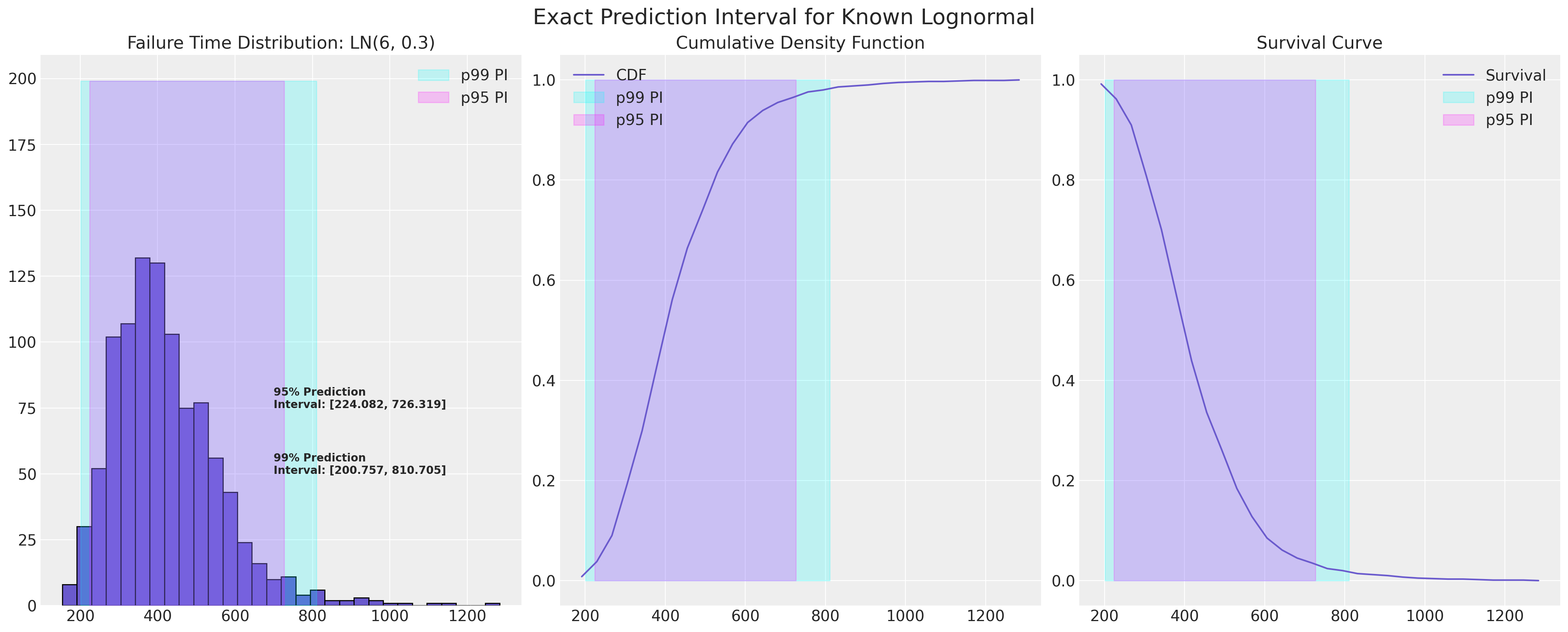
In the study of reliability statistics there is a focus on location-scale based distributions with long tails. In an ideal world we’d know exactly which distribution described our failure process and the prediction interval for the next failure could be defined exactly.
mu, sigma = 6, 0.3


def plot_ln_pi(mu, sigma, xy=(700, 75), title="Exact Prediction Interval for Known Lognormal"):
    failure_dist = lognorm(s=sigma, scale=np.exp(mu))
    samples = failure_dist.rvs(size=1000, random_state=100)
    fig, axs = plt.subplots(1, 3, figsize=(20, 8))
    axs = axs.flatten()
    axs[0].hist(samples, ec="black", color="slateblue", bins=30)
    axs[0].set_title(f"Failure Time Distribution: LN({mu}, {sigma})")
    count, bins_count = np.histogram(samples, bins=30)
    pdf = count / sum(count)
    cdf = np.cumsum(pdf)
    axs[1].plot(bins_count[1:], cdf, label="CDF", color="slateblue")
    axs[2].plot(bins_count[1:], 1 - cdf, label="Survival", color="slateblue")
    axs[2].legend()
    axs[1].legend()
    axs[1].set_title("Cumulative Density Function")
    axs[2].set_title("Survival Curve")

    lb = failure_dist.ppf(0.01)
    ub = failure_dist.ppf(0.99)
    axs[0].annotate(
        f"99% Prediction \nInterval: [{np.round(lb, 3)}, {np.round(ub, 3)}]",
        xy=(xy[0], xy[1] - 25),
        fontweight="bold",
    )
    axs[0].fill_betweenx(y=range(200), x1=lb, x2=ub, alpha=0.2, label="p99 PI", color="cyan")
    axs[1].fill_betweenx(y=range(2), x1=lb, x2=ub, alpha=0.2, label="p99 PI", color="cyan")
    axs[2].fill_betweenx(y=range(2), x1=lb, x2=ub, alpha=0.2, label="p99 PI", color="cyan")
    lb = failure_dist.ppf(0.025)
    ub = failure_dist.ppf(0.975)
    axs[0].annotate(
        f"95% Prediction \nInterval: [{np.round(lb, 3)}, {np.round(ub, 3)}]",
        xy=(xy[0], xy[1]),
        fontweight="bold",
    )
    axs[0].fill_betweenx(y=range(200), x1=lb, x2=ub, alpha=0.2, label="p95 PI", color="magenta")
    axs[1].fill_betweenx(y=range(2), x1=lb, x2=ub, alpha=0.2, label="p95 PI", color="magenta")
    axs[2].fill_betweenx(y=range(2), x1=lb, x2=ub, alpha=0.2, label="p95 PI", color="magenta")
    axs[0].legend()
    axs[1].legend()
    axs[2].legend()
    plt.suptitle(title, fontsize=20)


plot_ln_pi(mu, sigma)
Estimation of the Failure Distribution from Data#
In the real world we rarely have such exact knowledge. Instead we start with altogether less clear data. We will first examine failure data about heat exchanges across three plants and pool the information to quantify the lifetime of the heat-exchanges over the three factories.
The data is small deliberately so we can focus on the descriptive statistics involved in assessing time-to-failure data. In particular we’ll estimate the empirical CDF and survival functions. We will then generalise this style of analysis to a larger data set afterwards.
Heat Exchange Data#
Note on Censored Data: See below how the failure data flags whether or not an observation has been censored i.e. whether or not we have observed the full course of the life-time of the heat-exchanger. This is a crucial feature of failure time data. Too simple a statistical summary will be biased in its estimation of the prevalance of failure by the fact that our study has not seen out the full-course of every item’s life-cycle. The most prevalent form of censoring is so called “Right censored” data where we have not seen the “failure” event for a subset of the observations. Our histories are incomplete due to prematurely ending the data collection.
Left censoring (where we don’t observe an item from the beginning of their history) and interval censoring (both left and right censoring) can also occur but are less common.
Show code cell source
heat_exchange_df = pd.read_csv(
    StringIO(
        """Years Lower,Years Upper,Censoring Indicator,Count,Plant
0,1,Left,1,1
1,2,Interval,2,1
2,3,Interval,2,1
3, ,Right,95,1
0,1,Left,2,2
1,2,Interval,3,2
2, ,Right,95,2
0,1,Left,1,3
1, ,Right,99,3

"""
    )
)

heat_exchange_df["year_interval"] = (
    heat_exchange_df["Years Lower"].astype(str) + "," + heat_exchange_df["Years Upper"].astype(str)
)
heat_exchange_df["failed"] = np.where(
    heat_exchange_df["Censoring Indicator"] != "Right", heat_exchange_df["Count"], 0
)
heat_exchange_df["censored"] = np.where(
    heat_exchange_df["Censoring Indicator"] == "Right", heat_exchange_df["Count"], 0
)
heat_exchange_df["risk_set"] = [100, 99, 97, 0, 100, 98, 0, 100, 0]
heat_exchange_df
| Years Lower | Years Upper | Censoring Indicator | Count | Plant | year_interval | failed | censored | risk_set | |
|---|---|---|---|---|---|---|---|---|---|
| 0 | 0 | 1 | Left | 1 | 1 | 0,1 | 1 | 0 | 100 |
| 1 | 1 | 2 | Interval | 2 | 1 | 1,2 | 2 | 0 | 99 |
| 2 | 2 | 3 | Interval | 2 | 1 | 2,3 | 2 | 0 | 97 |
| 3 | 3 | Right | 95 | 1 | 3, | 0 | 95 | 0 | |
| 4 | 0 | 1 | Left | 2 | 2 | 0,1 | 2 | 0 | 100 |
| 5 | 1 | 2 | Interval | 3 | 2 | 1,2 | 3 | 0 | 98 |
| 6 | 2 | Right | 95 | 2 | 2, | 0 | 95 | 0 | |
| 7 | 0 | 1 | Left | 1 | 3 | 0,1 | 1 | 0 | 100 |
| 8 | 1 | Right | 99 | 3 | 1, | 0 | 99 | 0 |
actuarial_table = heat_exchange_df.groupby(["Years Upper"])[["failed", "risk_set"]].sum()
actuarial_table = actuarial_table.tail(3)


def greenwood_variance(df):
    ### Used to estimate the variance in the CDF
    n = len(df)
    ps = [df.iloc[i]["p_hat"] / (df.iloc[i]["risk_set"] * df.iloc[i]["1-p_hat"]) for i in range(n)]
    s = [(df.iloc[i]["S_hat"] ** 2) * np.sum(ps[0 : i + 1]) for i in range(n)]
    return s


def logit_transform_interval(df):
    ### Used for robustness in the estimation of the Confidence intervals in the CDF
    df["logit_CI_95_lb"] = df["F_hat"] / (
        df["F_hat"]
        + df["S_hat"] * np.exp((1.960 * df["Standard_Error"]) / (df["F_hat"] * df["S_hat"]))
    )
    df["logit_CI_95_ub"] = df["F_hat"] / (
        df["F_hat"]
        + df["S_hat"] / np.exp((1.960 * df["Standard_Error"]) / (df["F_hat"] * df["S_hat"]))
    )
    df["logit_CI_95_lb"] = np.where(df["logit_CI_95_lb"] < 0, 0, df["logit_CI_95_lb"])
    df["logit_CI_95_ub"] = np.where(df["logit_CI_95_ub"] > 1, 1, df["logit_CI_95_ub"])
    return df


def make_actuarial_table(actuarial_table):
    ### Actuarial lifetables are used to describe the nature of the risk over time and estimate
    actuarial_table["p_hat"] = actuarial_table["failed"] / actuarial_table["risk_set"]
    actuarial_table["1-p_hat"] = 1 - actuarial_table["p_hat"]
    actuarial_table["S_hat"] = actuarial_table["1-p_hat"].cumprod()
    actuarial_table["CH_hat"] = -np.log(actuarial_table["S_hat"])
    ### The Estimate of the CDF function
    actuarial_table["F_hat"] = 1 - actuarial_table["S_hat"]
    actuarial_table["V_hat"] = greenwood_variance(actuarial_table)
    actuarial_table["Standard_Error"] = np.sqrt(actuarial_table["V_hat"])
    actuarial_table["CI_95_lb"] = (
        actuarial_table["F_hat"] - actuarial_table["Standard_Error"] * 1.960
    )
    actuarial_table["CI_95_lb"] = np.where(
        actuarial_table["CI_95_lb"] < 0, 0, actuarial_table["CI_95_lb"]
    )
    actuarial_table["CI_95_ub"] = (
        actuarial_table["F_hat"] + actuarial_table["Standard_Error"] * 1.960
    )
    actuarial_table["CI_95_ub"] = np.where(
        actuarial_table["CI_95_ub"] > 1, 1, actuarial_table["CI_95_ub"]
    )
    actuarial_table["ploting_position"] = actuarial_table["F_hat"].rolling(1).median()
    actuarial_table = logit_transform_interval(actuarial_table)
    return actuarial_table


actuarial_table_heat = make_actuarial_table(actuarial_table)
actuarial_table_heat = actuarial_table_heat.reset_index()
actuarial_table_heat.rename({"Years Upper": "t"}, axis=1, inplace=True)
actuarial_table_heat["t"] = actuarial_table_heat["t"].astype(int)
actuarial_table_heat
| t | failed | risk_set | p_hat | 1-p_hat | S_hat | CH_hat | F_hat | V_hat | Standard_Error | CI_95_lb | CI_95_ub | ploting_position | logit_CI_95_lb | logit_CI_95_ub | |
|---|---|---|---|---|---|---|---|---|---|---|---|---|---|---|---|
| 0 | 1 | 4 | 300 | 0.013333 | 0.986667 | 0.986667 | 0.013423 | 0.013333 | 0.000044 | 0.006622 | 0.000354 | 0.026313 | 0.013333 | 0.005013 | 0.034977 |
| 1 | 2 | 5 | 197 | 0.025381 | 0.974619 | 0.961624 | 0.039131 | 0.038376 | 0.000164 | 0.012802 | 0.013283 | 0.063468 | 0.038376 | 0.019818 | 0.073016 |
| 2 | 3 | 2 | 97 | 0.020619 | 0.979381 | 0.941797 | 0.059965 | 0.058203 | 0.000350 | 0.018701 | 0.021550 | 0.094856 | 0.058203 | 0.030694 | 0.107629 |
It’s worth taking some time to walk through this example because it establishes estimates of some key quantities in time-to-failure modelling.
First note how we’re treating time as a series of discrete intervals. The data format is in discrete period format, since it records aggregate failures over time. We’ll see below another format of failure data - the item-period format which records each individual item over all periods and their corresponding status. In this format the key quantities are the set of failed items and the risk_set in each period. Everything else is derived from these facts.
First we’ve established across all three companies in three consecutive years the number of heat-exchanges that were produced and subsequently failed. This provides an estimate of the probability of failure in the year: p_hat and its inverse 1-p_hat respectively. These are further combined over the course of the year to estimate the survival curve S_hat which can be further transformed to recover estimates of the cumulative hazard CH_hat and the cumulative density function F_hat.
Next we want a quick a dirty way to quantify the extent of the uncertainty in our estimate of the CDF. For this purpose we use greenwood’s formula to estimate the variance of our V_hat of our estimate F_hat. This gives us the standard error and the two varieties of confidence interval recommended in the literature.
We’ apply the same techniques to a larger dataset and plot some of these quantities below.
The Shock Absorbers Data: A Study in Frequentist Reliability Analysis#
The shock absorbers data is in period format but it records a constantly decreasing risk set over time with one item being censored or failing at each time point i.e. removed from testing successfully (approved) or removed due to failure. This is a special case of the period format data.
Show code cell source
shockabsorbers_df = pd.read_csv(
    StringIO(
        """Kilometers,Failure Mode,Censoring Indicator
6700,Mode1,Failed
6950,Censored,Censored
7820,Censored,Censored
8790,Censored,Censored
9120,Mode2,Failed
9660,Censored,Censored
9820,Censored,Censored
11310,Censored,Censored
11690,Censored,Censored
11850,Censored,Censored
11880,Censored,Censored
12140,Censored,Censored
12200,Mode1,Failed
12870,Censored,Censored
13150,Mode2,Failed
13330,Censored,Censored
13470,Censored,Censored
14040,Censored,Censored
14300,Mode1,Failed
17520,Mode1,Failed
17540,Censored,Censored
17890,Censored,Censored
18450,Censored,Censored
18960,Censored,Censored
18980,Censored,Censored
19410,Censored,Censored
20100,Mode2,Failed
20100,Censored,Censored
20150,Censored,Censored
20320,Censored,Censored
20900,Mode2,Failed
22700,Mode1,Failed
23490,Censored,Censored
26510,Mode1,Failed
27410,Censored,Censored
27490,Mode1,Failed
27890,Censored,Censored
28100,Censored,Censored
"""
    )
)

shockabsorbers_df["failed"] = np.where(shockabsorbers_df["Censoring Indicator"] == "Failed", 1, 0)
shockabsorbers_df["t"] = shockabsorbers_df["Kilometers"]
shockabsorbers_events = survival_table_from_events(
    shockabsorbers_df["t"], shockabsorbers_df["failed"]
).reset_index()
shockabsorbers_events.rename(
    {"event_at": "t", "observed": "failed", "at_risk": "risk_set"}, axis=1, inplace=True
)
actuarial_table_shock = make_actuarial_table(shockabsorbers_events)
actuarial_table_shock
| t | removed | failed | censored | entrance | risk_set | p_hat | 1-p_hat | S_hat | CH_hat | F_hat | V_hat | Standard_Error | CI_95_lb | CI_95_ub | ploting_position | logit_CI_95_lb | logit_CI_95_ub | |
|---|---|---|---|---|---|---|---|---|---|---|---|---|---|---|---|---|---|---|
| 0 | 0.0 | 0 | 0 | 0 | 38 | 38 | 0.000000 | 1.000000 | 1.000000 | -0.000000 | 0.000000 | 0.000000 | 0.000000 | 0.000000 | 0.000000 | 0.000000 | NaN | NaN |
| 1 | 6700.0 | 1 | 1 | 0 | 0 | 38 | 0.026316 | 0.973684 | 0.973684 | 0.026668 | 0.026316 | 0.000674 | 0.025967 | 0.000000 | 0.077212 | 0.026316 | 0.003694 | 0.164570 |
| 2 | 6950.0 | 1 | 0 | 1 | 0 | 37 | 0.000000 | 1.000000 | 0.973684 | 0.026668 | 0.026316 | 0.000674 | 0.025967 | 0.000000 | 0.077212 | 0.026316 | 0.003694 | 0.164570 |
| 3 | 7820.0 | 1 | 0 | 1 | 0 | 36 | 0.000000 | 1.000000 | 0.973684 | 0.026668 | 0.026316 | 0.000674 | 0.025967 | 0.000000 | 0.077212 | 0.026316 | 0.003694 | 0.164570 |
| 4 | 8790.0 | 1 | 0 | 1 | 0 | 35 | 0.000000 | 1.000000 | 0.973684 | 0.026668 | 0.026316 | 0.000674 | 0.025967 | 0.000000 | 0.077212 | 0.026316 | 0.003694 | 0.164570 |
| 5 | 9120.0 | 1 | 1 | 0 | 0 | 34 | 0.029412 | 0.970588 | 0.945046 | 0.056521 | 0.054954 | 0.001431 | 0.037831 | 0.000000 | 0.129103 | 0.054954 | 0.013755 | 0.195137 |
| 6 | 9660.0 | 1 | 0 | 1 | 0 | 33 | 0.000000 | 1.000000 | 0.945046 | 0.056521 | 0.054954 | 0.001431 | 0.037831 | 0.000000 | 0.129103 | 0.054954 | 0.013755 | 0.195137 |
| 7 | 9820.0 | 1 | 0 | 1 | 0 | 32 | 0.000000 | 1.000000 | 0.945046 | 0.056521 | 0.054954 | 0.001431 | 0.037831 | 0.000000 | 0.129103 | 0.054954 | 0.013755 | 0.195137 |
| 8 | 11310.0 | 1 | 0 | 1 | 0 | 31 | 0.000000 | 1.000000 | 0.945046 | 0.056521 | 0.054954 | 0.001431 | 0.037831 | 0.000000 | 0.129103 | 0.054954 | 0.013755 | 0.195137 |
| 9 | 11690.0 | 1 | 0 | 1 | 0 | 30 | 0.000000 | 1.000000 | 0.945046 | 0.056521 | 0.054954 | 0.001431 | 0.037831 | 0.000000 | 0.129103 | 0.054954 | 0.013755 | 0.195137 |
| 10 | 11850.0 | 1 | 0 | 1 | 0 | 29 | 0.000000 | 1.000000 | 0.945046 | 0.056521 | 0.054954 | 0.001431 | 0.037831 | 0.000000 | 0.129103 | 0.054954 | 0.013755 | 0.195137 |
| 11 | 11880.0 | 1 | 0 | 1 | 0 | 28 | 0.000000 | 1.000000 | 0.945046 | 0.056521 | 0.054954 | 0.001431 | 0.037831 | 0.000000 | 0.129103 | 0.054954 | 0.013755 | 0.195137 |
| 12 | 12140.0 | 1 | 0 | 1 | 0 | 27 | 0.000000 | 1.000000 | 0.945046 | 0.056521 | 0.054954 | 0.001431 | 0.037831 | 0.000000 | 0.129103 | 0.054954 | 0.013755 | 0.195137 |
| 13 | 12200.0 | 1 | 1 | 0 | 0 | 26 | 0.038462 | 0.961538 | 0.908698 | 0.095742 | 0.091302 | 0.002594 | 0.050927 | 0.000000 | 0.191119 | 0.091302 | 0.029285 | 0.250730 |
| 14 | 12870.0 | 1 | 0 | 1 | 0 | 25 | 0.000000 | 1.000000 | 0.908698 | 0.095742 | 0.091302 | 0.002594 | 0.050927 | 0.000000 | 0.191119 | 0.091302 | 0.029285 | 0.250730 |
| 15 | 13150.0 | 1 | 1 | 0 | 0 | 24 | 0.041667 | 0.958333 | 0.870836 | 0.138302 | 0.129164 | 0.003756 | 0.061285 | 0.009046 | 0.249282 | 0.129164 | 0.048510 | 0.301435 |
| 16 | 13330.0 | 1 | 0 | 1 | 0 | 23 | 0.000000 | 1.000000 | 0.870836 | 0.138302 | 0.129164 | 0.003756 | 0.061285 | 0.009046 | 0.249282 | 0.129164 | 0.048510 | 0.301435 |
| 17 | 13470.0 | 1 | 0 | 1 | 0 | 22 | 0.000000 | 1.000000 | 0.870836 | 0.138302 | 0.129164 | 0.003756 | 0.061285 | 0.009046 | 0.249282 | 0.129164 | 0.048510 | 0.301435 |
| 18 | 14040.0 | 1 | 0 | 1 | 0 | 21 | 0.000000 | 1.000000 | 0.870836 | 0.138302 | 0.129164 | 0.003756 | 0.061285 | 0.009046 | 0.249282 | 0.129164 | 0.048510 | 0.301435 |
| 19 | 14300.0 | 1 | 1 | 0 | 0 | 20 | 0.050000 | 0.950000 | 0.827294 | 0.189595 | 0.172706 | 0.005191 | 0.072047 | 0.031495 | 0.313917 | 0.172706 | 0.072098 | 0.359338 |
| 20 | 17520.0 | 1 | 1 | 0 | 0 | 19 | 0.052632 | 0.947368 | 0.783752 | 0.243662 | 0.216248 | 0.006455 | 0.080342 | 0.058778 | 0.373717 | 0.216248 | 0.098254 | 0.411308 |
| 21 | 17540.0 | 1 | 0 | 1 | 0 | 18 | 0.000000 | 1.000000 | 0.783752 | 0.243662 | 0.216248 | 0.006455 | 0.080342 | 0.058778 | 0.373717 | 0.216248 | 0.098254 | 0.411308 |
| 22 | 17890.0 | 1 | 0 | 1 | 0 | 17 | 0.000000 | 1.000000 | 0.783752 | 0.243662 | 0.216248 | 0.006455 | 0.080342 | 0.058778 | 0.373717 | 0.216248 | 0.098254 | 0.411308 |
| 23 | 18450.0 | 1 | 0 | 1 | 0 | 16 | 0.000000 | 1.000000 | 0.783752 | 0.243662 | 0.216248 | 0.006455 | 0.080342 | 0.058778 | 0.373717 | 0.216248 | 0.098254 | 0.411308 |
| 24 | 18960.0 | 1 | 0 | 1 | 0 | 15 | 0.000000 | 1.000000 | 0.783752 | 0.243662 | 0.216248 | 0.006455 | 0.080342 | 0.058778 | 0.373717 | 0.216248 | 0.098254 | 0.411308 |
| 25 | 18980.0 | 1 | 0 | 1 | 0 | 14 | 0.000000 | 1.000000 | 0.783752 | 0.243662 | 0.216248 | 0.006455 | 0.080342 | 0.058778 | 0.373717 | 0.216248 | 0.098254 | 0.411308 |
| 26 | 19410.0 | 1 | 0 | 1 | 0 | 13 | 0.000000 | 1.000000 | 0.783752 | 0.243662 | 0.216248 | 0.006455 | 0.080342 | 0.058778 | 0.373717 | 0.216248 | 0.098254 | 0.411308 |
| 27 | 20100.0 | 2 | 1 | 1 | 0 | 12 | 0.083333 | 0.916667 | 0.718440 | 0.330673 | 0.281560 | 0.009334 | 0.096613 | 0.092199 | 0.470922 | 0.281560 | 0.133212 | 0.499846 |
| 28 | 20150.0 | 1 | 0 | 1 | 0 | 10 | 0.000000 | 1.000000 | 0.718440 | 0.330673 | 0.281560 | 0.009334 | 0.096613 | 0.092199 | 0.470922 | 0.281560 | 0.133212 | 0.499846 |
| 29 | 20320.0 | 1 | 0 | 1 | 0 | 9 | 0.000000 | 1.000000 | 0.718440 | 0.330673 | 0.281560 | 0.009334 | 0.096613 | 0.092199 | 0.470922 | 0.281560 | 0.133212 | 0.499846 |
| 30 | 20900.0 | 1 | 1 | 0 | 0 | 8 | 0.125000 | 0.875000 | 0.628635 | 0.464205 | 0.371365 | 0.014203 | 0.119177 | 0.137778 | 0.604953 | 0.371365 | 0.178442 | 0.616380 |
| 31 | 22700.0 | 1 | 1 | 0 | 0 | 7 | 0.142857 | 0.857143 | 0.538830 | 0.618356 | 0.461170 | 0.017348 | 0.131711 | 0.203016 | 0.719324 | 0.461170 | 0.232453 | 0.707495 |
| 32 | 23490.0 | 1 | 0 | 1 | 0 | 6 | 0.000000 | 1.000000 | 0.538830 | 0.618356 | 0.461170 | 0.017348 | 0.131711 | 0.203016 | 0.719324 | 0.461170 | 0.232453 | 0.707495 |
| 33 | 26510.0 | 1 | 1 | 0 | 0 | 5 | 0.200000 | 0.800000 | 0.431064 | 0.841499 | 0.568936 | 0.020393 | 0.142806 | 0.289037 | 0.848835 | 0.568936 | 0.296551 | 0.805150 |
| 34 | 27410.0 | 1 | 0 | 1 | 0 | 4 | 0.000000 | 1.000000 | 0.431064 | 0.841499 | 0.568936 | 0.020393 | 0.142806 | 0.289037 | 0.848835 | 0.568936 | 0.296551 | 0.805150 |
| 35 | 27490.0 | 1 | 1 | 0 | 0 | 3 | 0.333333 | 0.666667 | 0.287376 | 1.246964 | 0.712624 | 0.022828 | 0.151089 | 0.416490 | 1.000000 | 0.712624 | 0.368683 | 0.913267 |
| 36 | 27890.0 | 1 | 0 | 1 | 0 | 2 | 0.000000 | 1.000000 | 0.287376 | 1.246964 | 0.712624 | 0.022828 | 0.151089 | 0.416490 | 1.000000 | 0.712624 | 0.368683 | 0.913267 |
| 37 | 28100.0 | 1 | 0 | 1 | 0 | 1 | 0.000000 | 1.000000 | 0.287376 | 1.246964 | 0.712624 | 0.022828 | 0.151089 | 0.416490 | 1.000000 | 0.712624 | 0.368683 | 0.913267 |
Maximum Likelihood Fits for Failure Data#
In addition to taking descriptive summaries of our data we can use the life-table data to estimate a univariate model fit to our distribution of failure times. Such a fit, if good, would enable us to have a clearer view of the predictive distribution a particular set of predictive intervals. Here we’ll use the functions from the lifelines package to estimate the MLE fit on right-censored data.
lnf = LogNormalFitter().fit(actuarial_table_shock["t"] + 1e-25, actuarial_table_shock["failed"])
lnf.print_summary()
| model | lifelines.LogNormalFitter |
|---|---|
| number of observations | 38 |
| number of events observed | 11 |
| log-likelihood | -124.20 |
| hypothesis | mu_ != 0, sigma_ != 1 |
| coef | se(coef) | coef lower 95% | coef upper 95% | cmp to | z | p | -log2(p) | |
|---|---|---|---|---|---|---|---|---|
| mu_ | 10.13 | 0.14 | 9.85 | 10.41 | 0.00 | 71.08 | <0.005 | inf |
| sigma_ | 0.53 | 0.11 | 0.31 | 0.74 | 1.00 | -4.26 | <0.005 | 15.58 |
| AIC | 252.41 |
|---|
Although it’s tempting to take this model and run with it, we need to be cautious in the case of limited data. For instance in the heat-exchange data we have three years of data with a total of 11 failures. A too simple model can get this quite wrong. For the moment we’ll focus on the shock-absorber data - its non-parametric description and a simple univariate fit to this data.
Show code cell source
def plot_cdfs(actuarial_table, dist_fits=True, ax=None, title="", xy=(3000, 0.5), item_period=None):
    if item_period is None:
        lnf = LogNormalFitter().fit(actuarial_table["t"] + 1e-25, actuarial_table["failed"])
        wbf = WeibullFitter().fit(actuarial_table["t"] + 1e-25, actuarial_table["failed"])
    else:
        lnf = LogNormalFitter().fit(item_period["t"] + 1e-25, item_period["failed"])
        wbf = WeibullFitter().fit(item_period["t"] + 1e-25, item_period["failed"])
    if ax is None:
        fig, ax = plt.subplots(figsize=(20, 10))
    ax.plot(
        actuarial_table["t"],
        actuarial_table["F_hat"],
        "-o",
        color="black",
        label="Non-Parametric Estimate of CDF",
    )
    ax.plot(
        actuarial_table["t"],
        actuarial_table["CI_95_lb"],
        color="darkorchid",
        linestyle="--",
        label="Non-Parametric 95% CI based on Normal Approx",
    )
    ax.plot(actuarial_table["t"], actuarial_table["CI_95_ub"], color="darkorchid", linestyle="--")
    ax.fill_between(
        actuarial_table["t"].values,
        actuarial_table["CI_95_lb"].values,
        actuarial_table["CI_95_ub"].values,
        color="darkorchid",
        alpha=0.2,
    )
    ax.plot(
        actuarial_table["t"],
        actuarial_table["logit_CI_95_lb"],
        color="royalblue",
        linestyle="--",
        label="Non-Parametric 95% CI based on Logit Approx",
    )
    ax.plot(
        actuarial_table["t"], actuarial_table["logit_CI_95_ub"], color="royalblue", linestyle="--"
    )
    ax.fill_between(
        actuarial_table["t"].values,
        actuarial_table["logit_CI_95_lb"].values,
        actuarial_table["logit_CI_95_ub"].values,
        color="royalblue",
        alpha=0.2,
    )
    if dist_fits:
        lnf.plot_cumulative_density(ax=ax, color="crimson", alpha=0.8)
        wbf.plot_cumulative_density(ax=ax, color="cyan", alpha=0.8)
        ax.annotate(
            f"Lognormal Fit: mu = {np.round(lnf.mu_, 3)}, sigma = {np.round(lnf.sigma_, 3)} \nWeibull Fit: lambda = {np.round(wbf.lambda_, 3)}, rho = {np.round(wbf.rho_, 3)}",
            xy=(xy[0], xy[1]),
            fontsize=12,
            weight="bold",
        )
    ax.set_title(
        f"Estimates of the Cumulative Density Function \n derived from our {title} Failure Data",
        fontsize=20,
    )
    ax.set_ylabel("Fraction Failing")
    ax.set_xlabel("Time Scale")
    ax.legend()
    return ax
plot_cdfs(actuarial_table_shock, title="Shock Absorber");
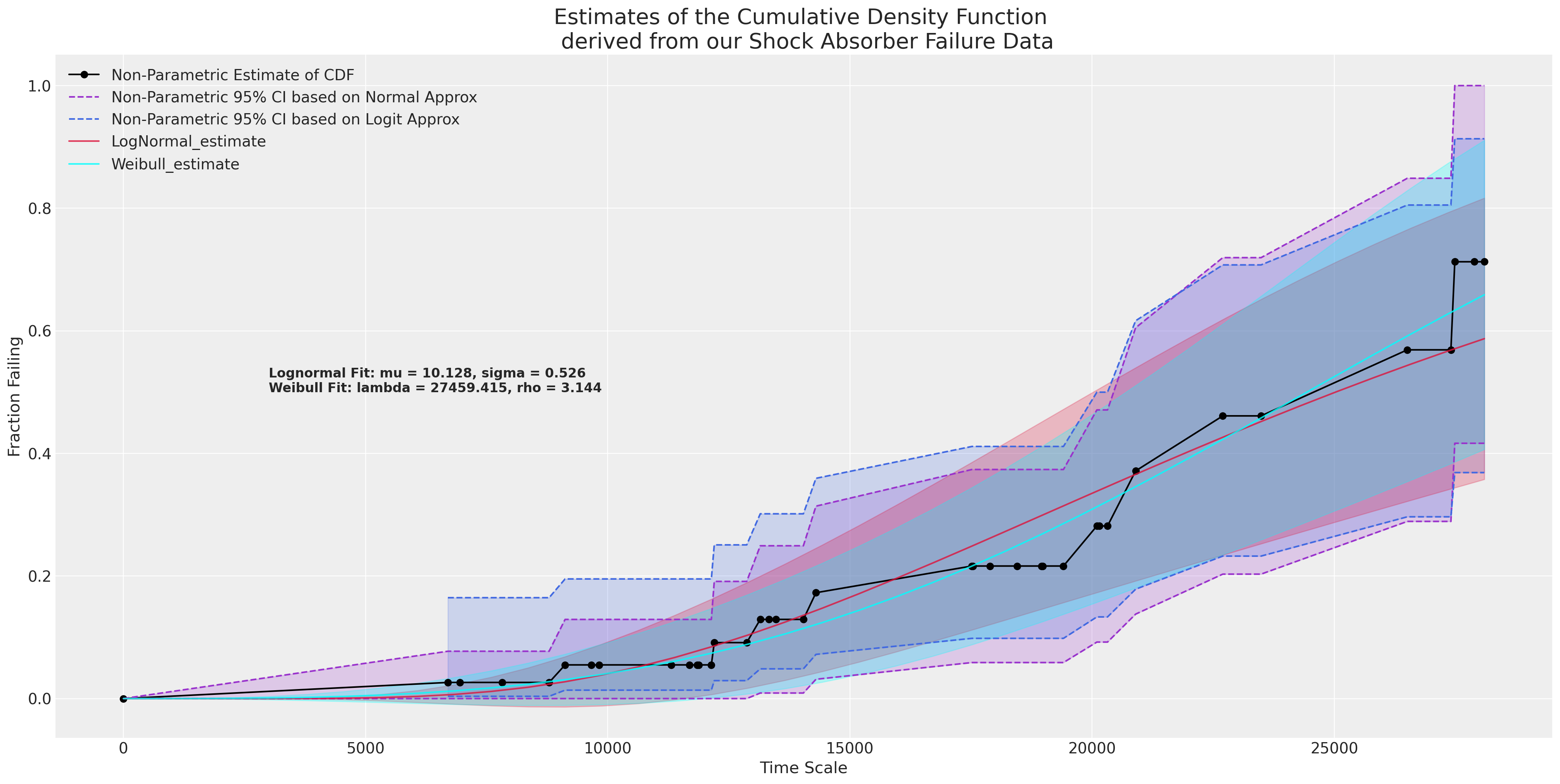
This shows a good fit to the data and implies, as you might expect, that the failing fraction of shock absorbers increases with age as they wear out. But how do we quantify the prediction given an estimated model?
The Plug-in-Procedure for calculating Approximate Statistical Prediction Intervals#
Since we’ve estimated a lognormal fit for the CDF of the shock absorbers data we can plot their approximate prediction interval. The interest here is likely to be in the lower bound of the prediction interval since we as manufacturers might want to be aware of warranty claims and the risk of exposure to refunds if the lower bound is too low.
plot_ln_pi(
    10.128,
    0.526,
    xy=(40000, 120),
    title="Plug-in Estimate of Shock Absorber Failure Prediction Interval",
)
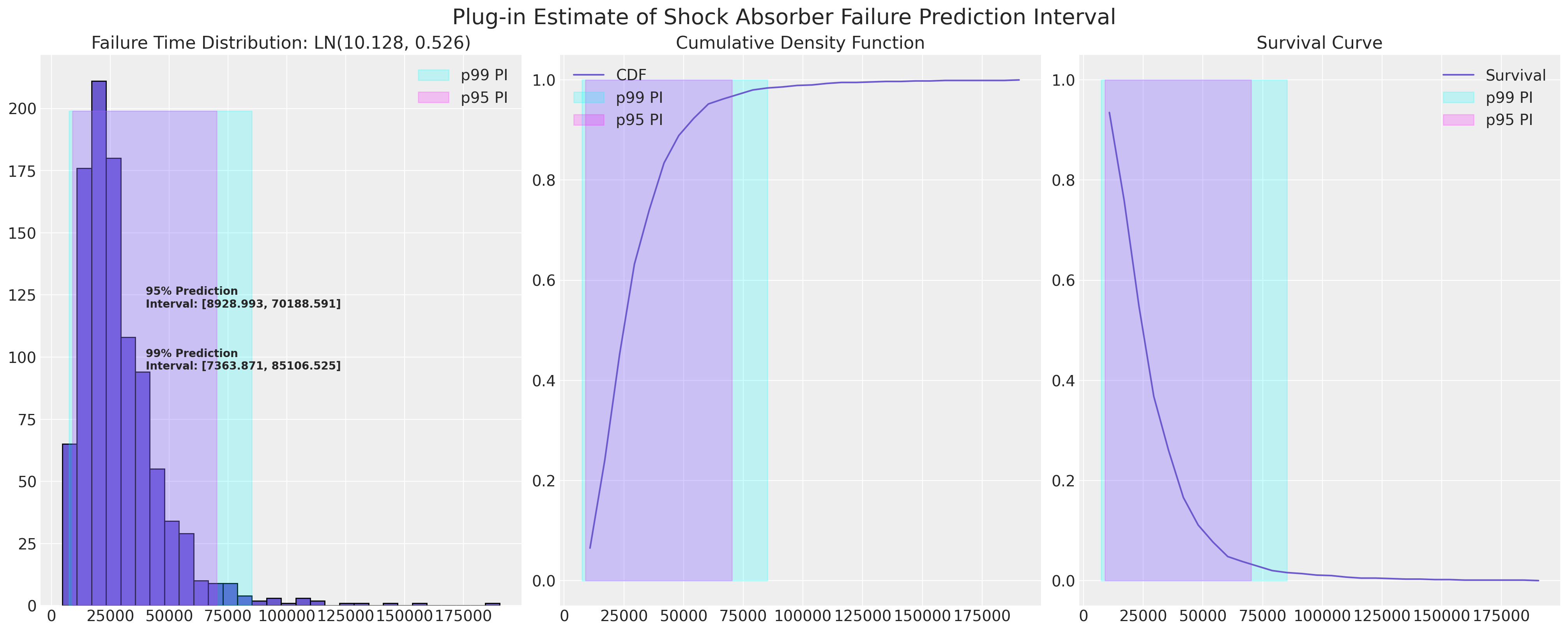
Bootstrap Calibration and Coverage Estimation#
We want now to estimate the coverage implied by this prediction interval, and to do so we will bootstrap estimates for the lower and upper bounds of the 95% confidence interval and ultimately assess their coverage conditional on the MLE fit. We will use the fractional weighted (bayesian) bootstrap. We’ll report two methods of estimating the coverage statistic - the first is the empirical coverage based on sampling a random value from within the known range and assess if it falls between the 95% MLE lower bound and upper bounds.
The second method we’ll use to assess coverage is to bootstrap estimates of a 95% lower bound and upper bound and then assess how much those bootstrapped values would cover conditional on the MLE fit.
def bayes_boot(df, lb, ub, seed=100):
    w = np.random.dirichlet(np.ones(len(df)), 1)[0]
    lnf = LogNormalFitter().fit(df["t"] + 1e-25, df["failed"], weights=w)
    rv = lognorm(s=lnf.sigma_, scale=np.exp(lnf.mu_))
    ## Sample random choice from implied bootstrapped distribution
    choices = rv.rvs(1000)
    future = random.choice(choices)
    ## Check if choice is contained within the MLE 95% PI
    contained = (future >= lb) & (future <= ub)
    ## Record 95% interval of bootstrapped dist
    lb = rv.ppf(0.025)
    ub = rv.ppf(0.975)
    return lb, ub, contained, future, lnf.sigma_, lnf.mu_
CIs = [bayes_boot(actuarial_table_shock, 8928, 70188, seed=i) for i in range(1000)]
draws = pd.DataFrame(
    CIs, columns=["Lower Bound PI", "Upper Bound PI", "Contained", "future", "Sigma", "Mu"]
)
draws
| Lower Bound PI | Upper Bound PI | Contained | future | Sigma | Mu | |
|---|---|---|---|---|---|---|
| 0 | 9539.612509 | 52724.144855 | True | 12721.873679 | 0.436136 | 10.018018 |
| 1 | 11190.287884 | 70193.514908 | True | 37002.708820 | 0.468429 | 10.240906 |
| 2 | 12262.816075 | 49883.853578 | True | 47419.786326 | 0.357947 | 10.115890 |
| 3 | 10542.933491 | 119175.518677 | False | 82191.111953 | 0.618670 | 10.475782 |
| 4 | 9208.478350 | 62352.752208 | True | 25393.072528 | 0.487938 | 10.084221 |
| ... | ... | ... | ... | ... | ... | ... |
| 995 | 9591.084003 | 85887.280659 | True | 53836.013839 | 0.559245 | 10.264690 |
| 996 | 9724.522689 | 45044.965713 | True | 19481.035376 | 0.391081 | 9.948911 |
| 997 | 8385.673724 | 104222.628035 | True | 16417.930907 | 0.642870 | 10.294282 |
| 998 | 11034.708453 | 56492.385175 | True | 42085.798578 | 0.416605 | 10.125331 |
| 999 | 9408.619310 | 51697.495907 | True | 19253.676200 | 0.434647 | 10.001273 |
1000 rows × 6 columns
We can use these bootstrapped statistics to further calculate quantities of the predictive distribution. In our case we could use the parametric CDF for our simple parametric model, but we’ll adopt the empirical cdf here to show how this technique can be used when we have more complicated models too.
def ecdf(sample):
    # convert sample to a numpy array, if it isn't already
    sample = np.atleast_1d(sample)

    # find the unique values and their corresponding counts
    quantiles, counts = np.unique(sample, return_counts=True)

    # take the cumulative sum of the counts and divide by the sample size to
    # get the cumulative probabilities between 0 and 1
    cumprob = np.cumsum(counts).astype(np.double) / sample.size

    return quantiles, cumprob


fig, axs = plt.subplots(1, 2, figsize=(20, 6))
axs = axs.flatten()
ax = axs[0]
ax1 = axs[1]
hist_data = []
for i in range(1000):
    samples = lognorm(s=draws.iloc[i]["Sigma"], scale=np.exp(draws.iloc[i]["Mu"])).rvs(1000)
    qe, pe = ecdf(samples)
    ax.plot(qe, pe, color="skyblue", alpha=0.2)
    lkup = dict(zip(pe, qe))
    hist_data.append([lkup[0.05]])
hist_data = pd.DataFrame(hist_data, columns=["p05"])
samples = lognorm(s=draws["Sigma"].mean(), scale=np.exp(draws["Mu"].mean())).rvs(1000)
qe, pe = ecdf(samples)
ax.plot(qe, pe, color="red", label="Expected CDF for Shock Absorbers Data")
ax.set_xlim(0, 30_000)
ax.set_title("Bootstrapped CDF functions for the Shock Absorbers Data", fontsize=20)
ax1.hist(hist_data["p05"], color="slateblue", ec="black", alpha=0.4, bins=30)
ax1.set_title("Estimate of Uncertainty in the 5% Failure Time", fontsize=20)
ax1.axvline(
    hist_data["p05"].quantile(0.025), color="cyan", label="Lower Bound CI for 5% failure time"
)
ax1.axvline(
    hist_data["p05"].quantile(0.975), color="cyan", label="Upper Bound CI for 5% failure time"
)
ax1.legend()
ax.legend();

Next we’ll plot the bootstrapped data and the two estimates of coverage we achieve conditional on the MLE fit. In other words when we want to assess the coverage of a prediction interval based on our MLE fit we can also bootstrap an estimate for this quantity.
Show code cell source
mosaic = """AABB
            CCCC"""
fig, axs = plt.subplot_mosaic(mosaic=mosaic, figsize=(20, 12))
mle_rv = lognorm(s=0.53, scale=np.exp(10.128))
axs = [axs[k] for k in axs.keys()]
axs[0].scatter(
    draws["Mu"],
    draws["Lower Bound PI"],
    c=draws["Contained"],
    cmap=cm.cool,
    alpha=0.3,
    label="Fits in MLE 95% CI",
)
axs[1].scatter(
    draws["Sigma"],
    draws["Lower Bound PI"],
    c=draws["Contained"],
    cmap=cm.cool,
    alpha=0.3,
    label="Fits in MLE 95% CI",
)
axs[0].set_title("Bootstrapped Mu against Bootstrapped 95% Lower Bound")
prop = draws["Contained"].sum() / len(draws)
axs[0].annotate(
    f"Estimated Prediction \nEmpirical Coverage \nBased on Sampling : {np.round(prop, 3)}",
    xy=(10.4, 12000),
    fontweight="bold",
)
axs[1].set_title("Bootstrapped Sigma against Bootstrapped 95% Lower Bound")
axs[0].legend()
axs[0].set_xlabel("Mu")
axs[1].set_xlabel("Sigma")
axs[0].set_ylabel("Estimated Lower 95% PI")
axs[1].legend()
axs[2].hist(
    mle_rv.cdf(draws["Lower Bound PI"]),
    bins=50,
    label="Bootstrap 95% LB",
    ec="k",
    color="royalblue",
    alpha=0.2,
)
axs[2].hist(
    mle_rv.cdf(draws["Upper Bound PI"]),
    bins=50,
    label="Bootstrap 95% UB",
    ec="k",
    color="darkorchid",
    alpha=0.2,
)
axs[2].hist(
    np.abs(mle_rv.cdf(draws["Lower Bound PI"]) - mle_rv.cdf(draws["Upper Bound PI"])),
    alpha=0.2,
    bins=50,
    color="slateblue",
    ec="black",
    label="Bootstrap Abs Diff",
)
axs[2].axvline(
    np.abs(mle_rv.cdf(draws["Lower Bound PI"]) - mle_rv.cdf(draws["Upper Bound PI"])).mean(),
    label="Expected Coverage",
)
axs[2].set_title("Difference in LB and UB | MLE(mu, sigma)")
axs[2].legend()

plug_in = np.abs(
    np.mean(mle_rv.cdf(draws["Lower Bound PI"])) - np.mean(mle_rv.cdf(draws["Upper Bound PI"]))
)
lb = np.round(draws["Lower Bound PI"].mean(), 3)
ub = np.round(draws["Upper Bound PI"].mean(), 3)
axs[2].annotate(
    f"Estimated Prediction Interval \n Coverage Based on Plug in Method : {np.round(plug_in, 3)} \n with [{lb, ub}]",
    xy=(0.6, 80),
    fontweight="bold",
);
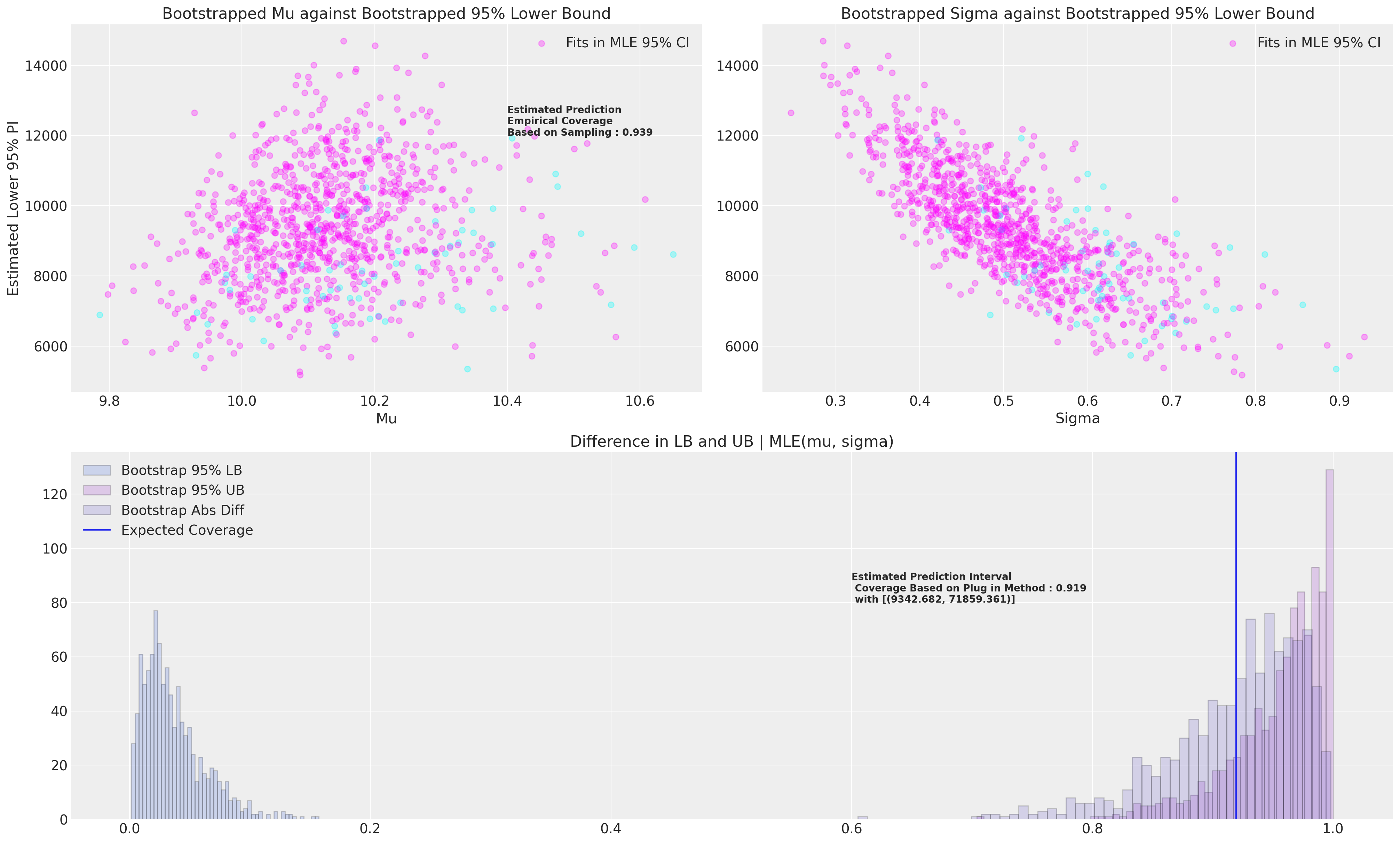
These simulations should be repeated a far larger number of times than we do here. It should be clear to see how we can also vary the MLE interval size to achieve the desired coverage level.
Bearing Cage Data: A Study in Bayesian Reliability Analysis#
Next we’ll look at a data set which has a slightly less clean parametric fit. The most obvious feature of this data is the small amount of failing records. The data is recorded in the period format with counts showing the extent of the risk set in each period.
We want to spend some time with this example to show how the frequentist techniques which worked well to estimate the shock-absorbers data can be augmented in the case of the Bearing cage data. In particular we’ll show how the issues arising can be resolved with a Bayesian approach.
Show code cell source
bearing_cage_df = pd.read_csv(
    StringIO(
        """Hours,Censoring Indicator,Count
50,Censored,288
150,Censored,148
230,Failed,1
250,Censored,124
334,Failed,1
350,Censored,111
423,Failed,1
450,Censored,106
550,Censored,99
650,Censored,110
750,Censored,114
850,Censored,119
950,Censored,127
990,Failed,1
1009,Failed,1
1050,Censored,123
1150,Censored,93
1250,Censored,47
1350,Censored,41
1450,Censored,27
1510,Failed,1
1550,Censored,11
1650,Censored,6
1850,Censored,1
2050,Censored,2"""
    )
)


bearing_cage_df["t"] = bearing_cage_df["Hours"]
bearing_cage_df["failed"] = np.where(bearing_cage_df["Censoring Indicator"] == "Failed", 1, 0)
bearing_cage_df["censored"] = np.where(
    bearing_cage_df["Censoring Indicator"] == "Censored", bearing_cage_df["Count"], 0
)
bearing_cage_events = survival_table_from_events(
    bearing_cage_df["t"], bearing_cage_df["failed"], weights=bearing_cage_df["Count"]
).reset_index()
bearing_cage_events.rename(
    {"event_at": "t", "observed": "failed", "at_risk": "risk_set"}, axis=1, inplace=True
)
actuarial_table_bearings = make_actuarial_table(bearing_cage_events)

actuarial_table_bearings
| t | removed | failed | censored | entrance | risk_set | p_hat | 1-p_hat | S_hat | CH_hat | F_hat | V_hat | Standard_Error | CI_95_lb | CI_95_ub | ploting_position | logit_CI_95_lb | logit_CI_95_ub | |
|---|---|---|---|---|---|---|---|---|---|---|---|---|---|---|---|---|---|---|
| 0 | 0.0 | 0 | 0 | 0 | 1703 | 1703 | 0.000000 | 1.000000 | 1.000000 | -0.000000 | 0.000000 | 0.000000e+00 | 0.000000 | 0.0 | 0.000000 | 0.000000 | NaN | NaN |
| 1 | 50.0 | 288 | 0 | 288 | 0 | 1703 | 0.000000 | 1.000000 | 1.000000 | -0.000000 | 0.000000 | 0.000000e+00 | 0.000000 | 0.0 | 0.000000 | 0.000000 | NaN | NaN |
| 2 | 150.0 | 148 | 0 | 148 | 0 | 1415 | 0.000000 | 1.000000 | 1.000000 | -0.000000 | 0.000000 | 0.000000e+00 | 0.000000 | 0.0 | 0.000000 | 0.000000 | NaN | NaN |
| 3 | 230.0 | 1 | 1 | 0 | 0 | 1267 | 0.000789 | 0.999211 | 0.999211 | 0.000790 | 0.000789 | 6.224491e-07 | 0.000789 | 0.0 | 0.002336 | 0.000789 | 0.000111 | 0.005581 |
| 4 | 250.0 | 124 | 0 | 124 | 0 | 1266 | 0.000000 | 1.000000 | 0.999211 | 0.000790 | 0.000789 | 6.224491e-07 | 0.000789 | 0.0 | 0.002336 | 0.000789 | 0.000111 | 0.005581 |
| 5 | 334.0 | 1 | 1 | 0 | 0 | 1142 | 0.000876 | 0.999124 | 0.998336 | 0.001666 | 0.001664 | 1.386254e-06 | 0.001177 | 0.0 | 0.003972 | 0.001664 | 0.000415 | 0.006641 |
| 6 | 350.0 | 111 | 0 | 111 | 0 | 1141 | 0.000000 | 1.000000 | 0.998336 | 0.001666 | 0.001664 | 1.386254e-06 | 0.001177 | 0.0 | 0.003972 | 0.001664 | 0.000415 | 0.006641 |
| 7 | 423.0 | 1 | 1 | 0 | 0 | 1030 | 0.000971 | 0.999029 | 0.997367 | 0.002637 | 0.002633 | 2.322113e-06 | 0.001524 | 0.0 | 0.005620 | 0.002633 | 0.000846 | 0.008165 |
| 8 | 450.0 | 106 | 0 | 106 | 0 | 1029 | 0.000000 | 1.000000 | 0.997367 | 0.002637 | 0.002633 | 2.322113e-06 | 0.001524 | 0.0 | 0.005620 | 0.002633 | 0.000846 | 0.008165 |
| 9 | 550.0 | 99 | 0 | 99 | 0 | 923 | 0.000000 | 1.000000 | 0.997367 | 0.002637 | 0.002633 | 2.322113e-06 | 0.001524 | 0.0 | 0.005620 | 0.002633 | 0.000846 | 0.008165 |
| 10 | 650.0 | 110 | 0 | 110 | 0 | 824 | 0.000000 | 1.000000 | 0.997367 | 0.002637 | 0.002633 | 2.322113e-06 | 0.001524 | 0.0 | 0.005620 | 0.002633 | 0.000846 | 0.008165 |
| 11 | 750.0 | 114 | 0 | 114 | 0 | 714 | 0.000000 | 1.000000 | 0.997367 | 0.002637 | 0.002633 | 2.322113e-06 | 0.001524 | 0.0 | 0.005620 | 0.002633 | 0.000846 | 0.008165 |
| 12 | 850.0 | 119 | 0 | 119 | 0 | 600 | 0.000000 | 1.000000 | 0.997367 | 0.002637 | 0.002633 | 2.322113e-06 | 0.001524 | 0.0 | 0.005620 | 0.002633 | 0.000846 | 0.008165 |
| 13 | 950.0 | 127 | 0 | 127 | 0 | 481 | 0.000000 | 1.000000 | 0.997367 | 0.002637 | 0.002633 | 2.322113e-06 | 0.001524 | 0.0 | 0.005620 | 0.002633 | 0.000846 | 0.008165 |
| 14 | 990.0 | 1 | 1 | 0 | 0 | 354 | 0.002825 | 0.997175 | 0.994549 | 0.005466 | 0.005451 | 1.022444e-05 | 0.003198 | 0.0 | 0.011718 | 0.005451 | 0.001722 | 0.017117 |
| 15 | 1009.0 | 1 | 1 | 0 | 0 | 353 | 0.002833 | 0.997167 | 0.991732 | 0.008303 | 0.008268 | 1.808196e-05 | 0.004252 | 0.0 | 0.016603 | 0.008268 | 0.003008 | 0.022519 |
| 16 | 1050.0 | 123 | 0 | 123 | 0 | 352 | 0.000000 | 1.000000 | 0.991732 | 0.008303 | 0.008268 | 1.808196e-05 | 0.004252 | 0.0 | 0.016603 | 0.008268 | 0.003008 | 0.022519 |
| 17 | 1150.0 | 93 | 0 | 93 | 0 | 229 | 0.000000 | 1.000000 | 0.991732 | 0.008303 | 0.008268 | 1.808196e-05 | 0.004252 | 0.0 | 0.016603 | 0.008268 | 0.003008 | 0.022519 |
| 18 | 1250.0 | 47 | 0 | 47 | 0 | 136 | 0.000000 | 1.000000 | 0.991732 | 0.008303 | 0.008268 | 1.808196e-05 | 0.004252 | 0.0 | 0.016603 | 0.008268 | 0.003008 | 0.022519 |
| 19 | 1350.0 | 41 | 0 | 41 | 0 | 89 | 0.000000 | 1.000000 | 0.991732 | 0.008303 | 0.008268 | 1.808196e-05 | 0.004252 | 0.0 | 0.016603 | 0.008268 | 0.003008 | 0.022519 |
| 20 | 1450.0 | 27 | 0 | 27 | 0 | 48 | 0.000000 | 1.000000 | 0.991732 | 0.008303 | 0.008268 | 1.808196e-05 | 0.004252 | 0.0 | 0.016603 | 0.008268 | 0.003008 | 0.022519 |
| 21 | 1510.0 | 1 | 1 | 0 | 0 | 21 | 0.047619 | 0.952381 | 0.944506 | 0.057093 | 0.055494 | 2.140430e-03 | 0.046265 | 0.0 | 0.146173 | 0.055494 | 0.010308 | 0.248927 |
| 22 | 1550.0 | 11 | 0 | 11 | 0 | 20 | 0.000000 | 1.000000 | 0.944506 | 0.057093 | 0.055494 | 2.140430e-03 | 0.046265 | 0.0 | 0.146173 | 0.055494 | 0.010308 | 0.248927 |
| 23 | 1650.0 | 6 | 0 | 6 | 0 | 9 | 0.000000 | 1.000000 | 0.944506 | 0.057093 | 0.055494 | 2.140430e-03 | 0.046265 | 0.0 | 0.146173 | 0.055494 | 0.010308 | 0.248927 |
| 24 | 1850.0 | 1 | 0 | 1 | 0 | 3 | 0.000000 | 1.000000 | 0.944506 | 0.057093 | 0.055494 | 2.140430e-03 | 0.046265 | 0.0 | 0.146173 | 0.055494 | 0.010308 | 0.248927 |
| 25 | 2050.0 | 2 | 0 | 2 | 0 | 2 | 0.000000 | 1.000000 | 0.944506 | 0.057093 | 0.055494 | 2.140430e-03 | 0.046265 | 0.0 | 0.146173 | 0.055494 | 0.010308 | 0.248927 |
To estimate a univariate or non-parametric CDF we need to disaggregate the period format data into an item-period format.
Item Period Data Format#
item_period = bearing_cage_df["Hours"].to_list() * bearing_cage_df["Count"].sum()
ids = [[i] * 25 for i in range(bearing_cage_df["Count"].sum())]
ids = [int(i) for l in ids for i in l]
item_period_bearing_cage = pd.DataFrame(item_period, columns=["t"])
item_period_bearing_cage["id"] = ids
item_period_bearing_cage["failed"] = np.zeros(len(item_period_bearing_cage))

## Censor appropriate number of ids
unique_ids = item_period_bearing_cage["id"].unique()
censored = bearing_cage_df[bearing_cage_df["Censoring Indicator"] == "Censored"]
i = 0
stack = []
for hour, count, idx in zip(censored["Hours"], censored["Count"], censored["Count"].cumsum()):
    temp = item_period_bearing_cage[
        item_period_bearing_cage["id"].isin(unique_ids[i:idx])
        & (item_period_bearing_cage["t"] == hour)
    ]
    stack.append(temp)
    i = idx

censored_clean = pd.concat(stack)

### Add  appropriate number of failings
stack = []
unique_times = censored_clean["t"].unique()
for id, fail_time in zip(
    [9999, 9998, 9997, 9996, 9995, 9994],
    bearing_cage_df[bearing_cage_df["failed"] == 1]["t"].values,
):
    temp = pd.DataFrame(unique_times[unique_times < fail_time], columns=["t"])
    temp["id"] = id
    temp["failed"] = 0
    temp = pd.concat([temp, pd.DataFrame({"t": [fail_time], "id": [id], "failed": [1]}, index=[0])])
    stack.append(temp)

failed_clean = pd.concat(stack).sort_values(["id", "t"])
censored_clean
item_period_bearing_cage = pd.concat([failed_clean, censored_clean])
## Transpose for more concise visual
item_period_bearing_cage.head(30).T
| 0 | 1 | 2 | 3 | 4 | 5 | 6 | 7 | 8 | 9 | ... | 4 | 5 | 6 | 7 | 8 | 9 | 0 | 0 | 1 | 2 | |
|---|---|---|---|---|---|---|---|---|---|---|---|---|---|---|---|---|---|---|---|---|---|
| t | 50.0 | 150.0 | 250.0 | 350.0 | 450.0 | 550.0 | 650.0 | 750.0 | 850.0 | 950.0 | ... | 450.0 | 550.0 | 650.0 | 750.0 | 850.0 | 950.0 | 1009.0 | 50.0 | 150.0 | 250.0 |
| id | 9994.0 | 9994.0 | 9994.0 | 9994.0 | 9994.0 | 9994.0 | 9994.0 | 9994.0 | 9994.0 | 9994.0 | ... | 9995.0 | 9995.0 | 9995.0 | 9995.0 | 9995.0 | 9995.0 | 9995.0 | 9996.0 | 9996.0 | 9996.0 |
| failed | 0.0 | 0.0 | 0.0 | 0.0 | 0.0 | 0.0 | 0.0 | 0.0 | 0.0 | 0.0 | ... | 0.0 | 0.0 | 0.0 | 0.0 | 0.0 | 0.0 | 1.0 | 0.0 | 0.0 | 0.0 |
3 rows × 30 columns
assert item_period_bearing_cage["id"].nunique() == 1703
assert item_period_bearing_cage["failed"].sum() == 6
assert item_period_bearing_cage[item_period_bearing_cage["t"] >= 1850]["id"].nunique() == 3
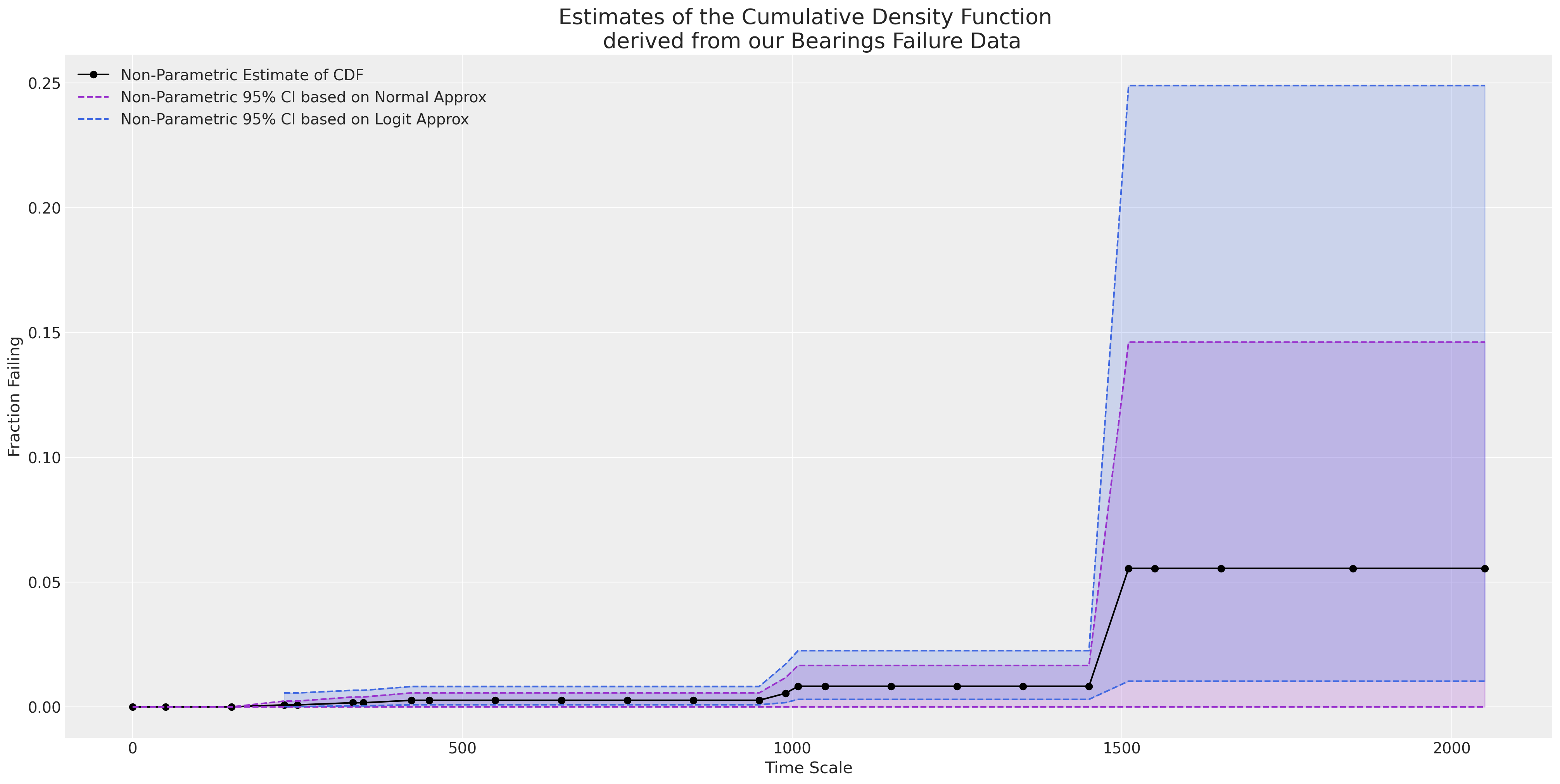
As we plot the empirical CDF we see that the y-axis only ever reaches as maximum height of 0.05. A naive MLE fit will go dramatically wrong in extrapolating outside the observed range of the data.
ax = plot_cdfs(
    actuarial_table_bearings,
    title="Bearings",
    dist_fits=False,
    xy=(20, 0.7),
    item_period=item_period_bearing_cage,
)
Probability Plots: Comparing CDFs in a Restricted Linear Range#
In this section we’ll use the technique of linearising the MLE fits so that can perform a visual “goodness of fit” check. These types of plots rely on a transformation that can be applied to the location and scale distributions to turn their CDF into a linear space.
For both the Lognormal and Weibull fits we can represent their CDF in a linear space as a relationship between the logged value t and an appropriate \(CDF^{-1}\).
Show code cell source
def sev_ppf(p):
    return np.log(-np.log(1 - p))


mosaic = """AABB
            CCCC"""
fig, axs = plt.subplot_mosaic(mosaic=mosaic, figsize=(20, 15))
axs = [axs[k] for k in axs.keys()]
ax = axs[0]
ax2 = axs[1]
ax3 = axs[2]
ax.plot(
    np.log(actuarial_table_bearings["t"]),
    norm.ppf(actuarial_table_bearings["logit_CI_95_ub"]),
    "-o",
    label="Non-Parametric CI UB",
    color="slateblue",
)
ax.scatter(
    np.log(actuarial_table_bearings["t"]),
    norm.ppf(actuarial_table_bearings["ploting_position"]),
    label="Non-Parametric CDF",
    color="black",
)
ax.plot(
    np.log(actuarial_table_bearings["t"]),
    norm.ppf(actuarial_table_bearings["logit_CI_95_lb"]),
    "-o",
    label="Non-Parametric CI LB",
    color="slateblue",
)
for mu in np.linspace(10, 12, 3):
    for sigma in np.linspace(1.6, 1.9, 3):
        rv = lognorm(s=sigma, scale=np.exp(mu))
        ax.plot(
            np.log(actuarial_table_bearings["t"]),
            norm.ppf(rv.cdf(actuarial_table_bearings["t"])),
            "--",
            label=f"LN({np.round(mu, 3)}, {np.round(sigma, 3)})",
            color="grey",
        )

lnf = LogNormalFitter().fit(item_period_bearing_cage["t"], item_period_bearing_cage["failed"])
rv = lognorm(s=lnf.sigma_, scale=np.exp(lnf.mu_))
ax.plot(
    np.log(actuarial_table_bearings["t"]),
    norm.ppf(rv.cdf(actuarial_table_bearings["t"])),
    "--",
    label=f"MLE LN({np.round(lnf.mu_, 3)}, {np.round(lnf.sigma_, 3)})",
    color="RED",
)

for r in np.linspace(1, 2, 3):
    for s in np.linspace(12000, 25000, 2):
        rv = weibull_min(c=r, scale=s)
        ax2.plot(
            np.log(actuarial_table_bearings["t"]),
            sev_ppf(rv.cdf(actuarial_table_bearings["t"])),
            "--",
            label=f"Wb({np.round(s, 3)}, {np.round(r, 3)})",
            color="lightblue",
        )


wbf = WeibullFitter().fit(item_period_bearing_cage["t"], item_period_bearing_cage["failed"])
rv = weibull_min(c=wbf.rho_, scale=wbf.lambda_)
ax2.plot(
    np.log(actuarial_table_bearings["t"]),
    sev_ppf(rv.cdf(actuarial_table_bearings["t"])),
    "--",
    label=f"MLE Wb({np.round(wbf.lambda_, 3)}, {np.round(wbf.rho_, 3)})",
    color="red",
)

ax2.plot(
    np.log(actuarial_table_bearings["t"]),
    sev_ppf(actuarial_table_bearings["logit_CI_95_ub"]),
    "-o",
    label="Non-Parametric CI UB",
    color="slateblue",
)
ax2.scatter(
    np.log(actuarial_table_bearings["t"]),
    sev_ppf(actuarial_table_bearings["ploting_position"]),
    label="Non-Parametric CDF",
    color="black",
)
ax2.plot(
    np.log(actuarial_table_bearings["t"]),
    sev_ppf(actuarial_table_bearings["logit_CI_95_lb"]),
    "-o",
    label="Non-Parametric CI LB",
    color="slateblue",
)

ax3.plot(
    actuarial_table_bearings["t"],
    actuarial_table_bearings["logit_CI_95_ub"],
    "-o",
    label="Non-Parametric CI UB",
    color="slateblue",
)
ax3.scatter(
    actuarial_table_bearings["t"],
    actuarial_table_bearings["F_hat"],
    label="Non-Parametric CDF",
    color="black",
)
ax3.plot(
    actuarial_table_bearings["t"],
    actuarial_table_bearings["logit_CI_95_lb"],
    "-o",
    label="Non-Parametric CI LB",
    color="slateblue",
)
lnf.plot_cumulative_density(ax=ax3, color="cyan")
wbf.plot_cumulative_density(ax=ax3, color="darkorchid")


ax2.set_title("Linearizing the Weibull CDF", fontsize=20)
ax.set_title("Linearizing the Lognormal CDF", fontsize=20)
ax3.set_title("MLE CDF Fits", fontsize=20)
ax.legend()
ax.set_xlabel("Time")
ax2.set_xlabel("Time")
xticks = np.round(np.linspace(0, actuarial_table_bearings["t"].max(), 10), 1)
yticks = np.round(np.linspace(0, actuarial_table_bearings["F_hat"].max(), 10), 4)
ax.set_xticklabels(xticks)
ax.set_yticklabels(yticks)
ax2.set_xticklabels(xticks)
ax2.set_yticklabels([])
ax2.legend()
ax.set_ylabel("Fraction Failing");
/home/oriol/bin/miniconda3/envs/releases/lib/python3.10/site-packages/pandas/core/arraylike.py:402: RuntimeWarning: divide by zero encountered in log
result = getattr(ufunc, method)(*inputs, **kwargs)
/home/oriol/bin/miniconda3/envs/releases/lib/python3.10/site-packages/pandas/core/arraylike.py:402: RuntimeWarning: divide by zero encountered in log
result = getattr(ufunc, method)(*inputs, **kwargs)
/tmp/ipykernel_29435/2628457585.py:2: RuntimeWarning: divide by zero encountered in log
return np.log(-np.log(1 - p))
/tmp/ipykernel_29435/2628457585.py:128: UserWarning: FixedFormatter should only be used together with FixedLocator
ax.set_xticklabels(xticks)
/tmp/ipykernel_29435/2628457585.py:129: UserWarning: FixedFormatter should only be used together with FixedLocator
ax.set_yticklabels(yticks)
/tmp/ipykernel_29435/2628457585.py:130: UserWarning: FixedFormatter should only be used together with FixedLocator
ax2.set_xticklabels(xticks)
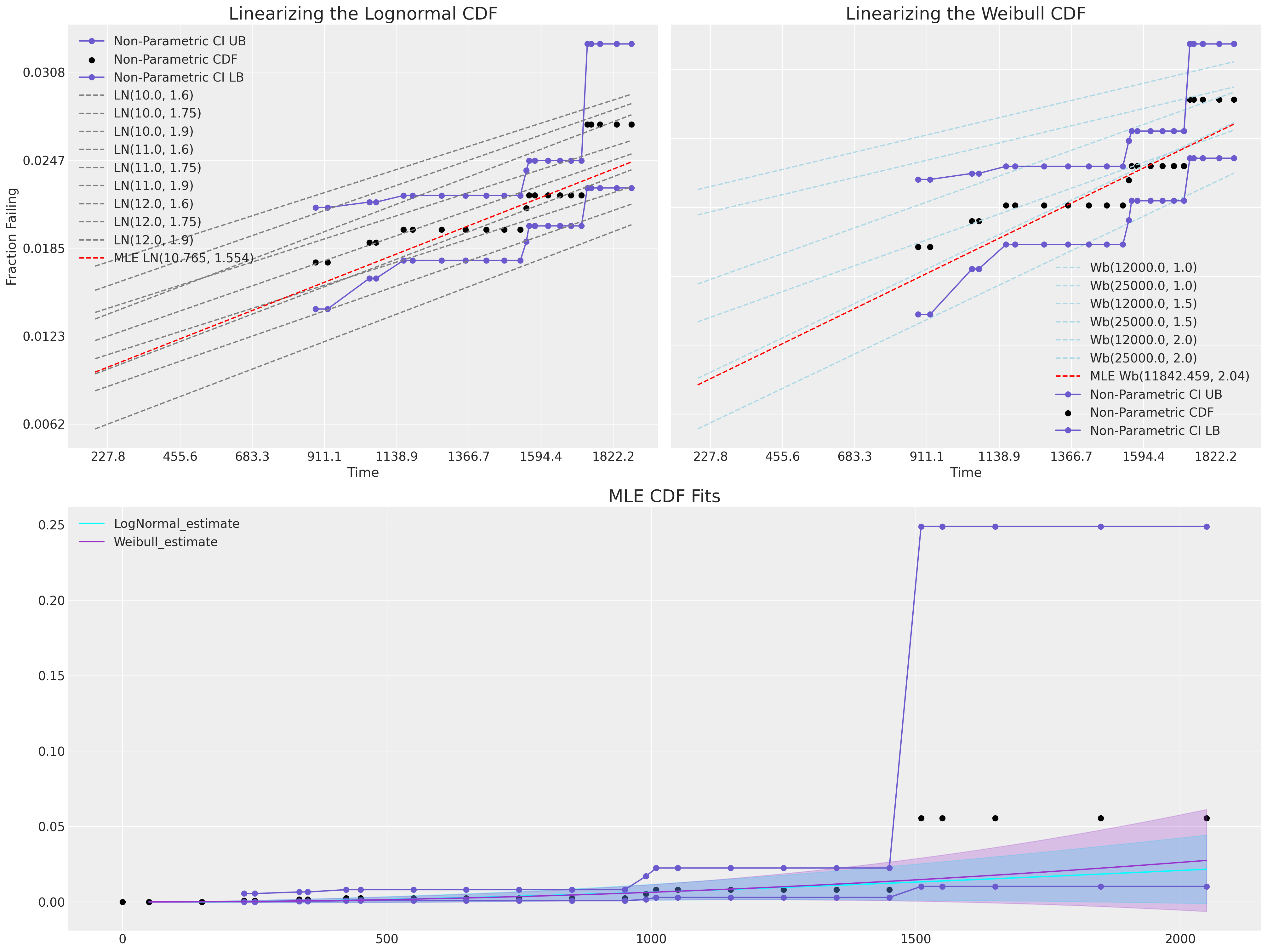
We can see here how neither MLE fit covers the range of observed data.
Bayesian Modelling of Reliability Data#
We’ve now seen how to model and visualise the parametric model fits to sparse reliability using a frequentist or MLE framework. We want to now show how the same style of inferences can be achieved in the Bayesian paradigm.
As in the MLE paradigm we need to model the censored liklihood. For most log-location distributions we’ve seen above the likelihood is expressed as a function of a combination of the distribution pdf \(\phi\) and cdf \(\Phi\) applied as appropriately depending on whether or not the data point was fully observed in the time window or censored.
where \(\delta_{i}\) is an indicator for whether the observation is a faiure or a right censored observation. More complicated types of censoring can be included with similar modifications of the CDF depending on the nature of the censored observations.
Direct PYMC implementation of Weibull Survival#
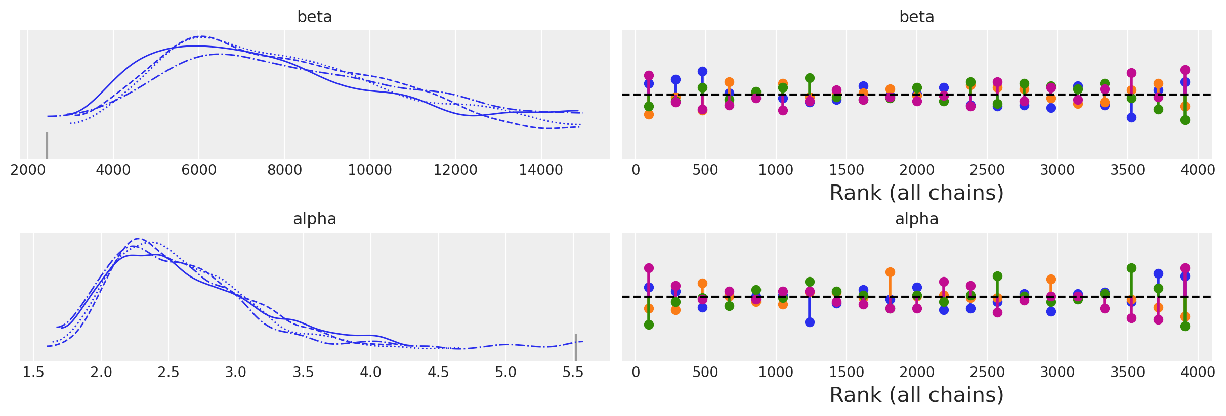
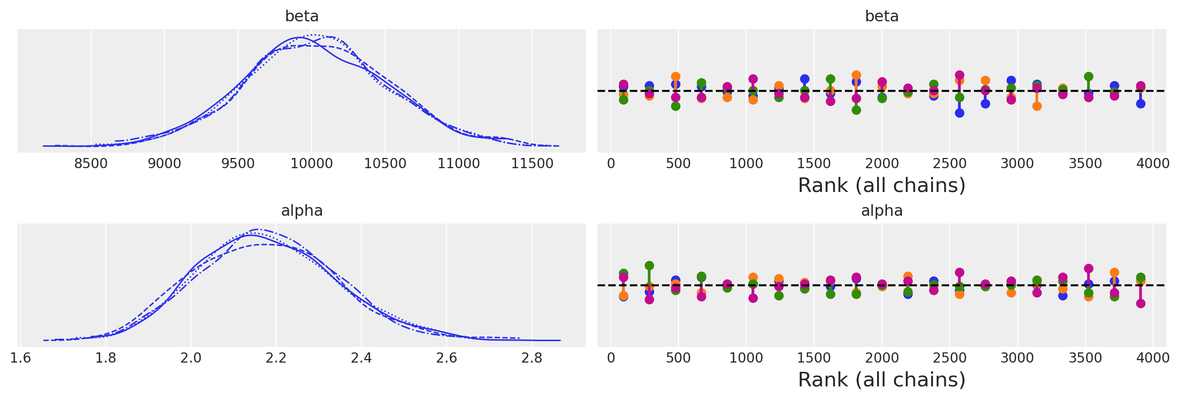
We fit two versions of this model with different specifications for the priors, one takes a vague uniform prior over the data, and another specifies priors closer to the MLE fits. We will show the implications of the prior specification has for the calibration of the model with the observed data below.
def weibull_lccdf(y, alpha, beta):
    """Log complementary cdf of Weibull distribution."""
    return -((y / beta) ** alpha)


item_period_max = item_period_bearing_cage.groupby("id")[["t", "failed"]].max()
y = item_period_max["t"].values
censored = ~item_period_max["failed"].values.astype(bool)


priors = {"beta": [100, 15_000], "alpha": [4, 1, 0.02, 8]}
priors_informative = {"beta": [10_000, 500], "alpha": [2, 0.5, 0.02, 3]}


def make_model(p, info=False):
    with pm.Model() as model:
        if info:
            beta = pm.Normal("beta", p["beta"][0], p["beta"][1])
        else:
            beta = pm.Uniform("beta", p["beta"][0], p["beta"][1])
        alpha = pm.TruncatedNormal(
            "alpha", p["alpha"][0], p["alpha"][1], lower=p["alpha"][2], upper=p["alpha"][3]
        )

        y_obs = pm.Weibull("y_obs", alpha=alpha, beta=beta, observed=y[~censored])
        y_cens = pm.Potential("y_cens", weibull_lccdf(y[censored], alpha, beta))
        idata = pm.sample_prior_predictive()
        idata.extend(pm.sample(random_seed=100, target_accept=0.95))
        idata.extend(pm.sample_posterior_predictive(idata))

    return idata, model


idata, model = make_model(priors)
idata_informative, model = make_model(priors_informative, info=True)
/tmp/ipykernel_29435/305144286.py:28: UserWarning: The effect of Potentials on other parameters is ignored during prior predictive sampling. This is likely to lead to invalid or biased predictive samples.
  idata = pm.sample_prior_predictive()
Sampling: [alpha, beta, y_obs]
Auto-assigning NUTS sampler...
Initializing NUTS using jitter+adapt_diag...
Multiprocess sampling (4 chains in 4 jobs)
NUTS: [beta, alpha]
Sampling 4 chains for 1_000 tune and 1_000 draw iterations (4_000 + 4_000 draws total) took 6 seconds.
/tmp/ipykernel_29435/305144286.py:30: UserWarning: The effect of Potentials on other parameters is ignored during posterior predictive sampling. This is likely to lead to invalid or biased predictive samples.
  idata.extend(pm.sample_posterior_predictive(idata))
Sampling: [y_obs]
idata
-
<xarray.Dataset> Dimensions: (chain: 4, draw: 1000) Coordinates: * chain (chain) int64 0 1 2 3 * draw (draw) int64 0 1 2 3 4 5 6 7 8 ... 992 993 994 995 996 997 998 999 Data variables: beta (chain, draw) float64 7.427e+03 8.514e+03 ... 1.013e+04 5.044e+03 alpha (chain, draw) float64 2.232 2.385 2.49 2.55 ... 2.437 2.503 2.898 Attributes: created_at: 2023-01-15T20:06:41.169437 arviz_version: 0.13.0 inference_library: pymc inference_library_version: 5.0.0 sampling_time: 6.423727989196777 tuning_steps: 1000 -
<xarray.Dataset> Dimensions: (chain: 4, draw: 1000, y_obs_dim_2: 6) Coordinates: * chain (chain) int64 0 1 2 3 * draw (draw) int64 0 1 2 3 4 5 6 7 ... 993 994 995 996 997 998 999 * y_obs_dim_2 (y_obs_dim_2) int64 0 1 2 3 4 5 Data variables: y_obs (chain, draw, y_obs_dim_2) float64 6.406e+03 ... 5.59e+03 Attributes: created_at: 2023-01-15T20:06:42.789072 arviz_version: 0.13.0 inference_library: pymc inference_library_version: 5.0.0 -
<xarray.Dataset> Dimensions: (chain: 4, draw: 1000) Coordinates: * chain (chain) int64 0 1 2 3 * draw (draw) int64 0 1 2 3 4 5 ... 994 995 996 997 998 999 Data variables: (12/17) perf_counter_diff (chain, draw) float64 0.0008238 ... 0.002601 n_steps (chain, draw) float64 3.0 3.0 7.0 ... 11.0 7.0 9.0 acceptance_rate (chain, draw) float64 0.9404 1.0 ... 0.9876 0.9424 smallest_eigval (chain, draw) float64 nan nan nan nan ... nan nan nan largest_eigval (chain, draw) float64 nan nan nan nan ... nan nan nan lp (chain, draw) float64 -80.96 -79.7 ... -81.05 -79.99 ... ... step_size_bar (chain, draw) float64 0.1791 0.1791 ... 0.1591 0.1591 reached_max_treedepth (chain, draw) bool False False False ... False False diverging (chain, draw) bool False False False ... False False process_time_diff (chain, draw) float64 0.0008239 ... 0.002601 index_in_trajectory (chain, draw) int64 -2 2 -3 -2 2 -2 ... -2 -1 -3 1 -6 perf_counter_start (chain, draw) float64 1.153e+04 ... 1.153e+04 Attributes: created_at: 2023-01-15T20:06:41.180463 arviz_version: 0.13.0 inference_library: pymc inference_library_version: 5.0.0 sampling_time: 6.423727989196777 tuning_steps: 1000 -
<xarray.Dataset> Dimensions: (chain: 1, draw: 500) Coordinates: * chain (chain) int64 0 * draw (draw) int64 0 1 2 3 4 5 6 7 8 ... 492 493 494 495 496 497 498 499 Data variables: alpha (chain, draw) float64 3.896 5.607 4.329 5.377 ... 3.828 4.875 3.723 beta (chain, draw) float64 6.915e+03 1.293e+04 ... 6.599e+03 1.244e+04 Attributes: created_at: 2023-01-15T20:06:29.497052 arviz_version: 0.13.0 inference_library: pymc inference_library_version: 5.0.0 -
<xarray.Dataset> Dimensions: (chain: 1, draw: 500, y_obs_dim_0: 6) Coordinates: * chain (chain) int64 0 * draw (draw) int64 0 1 2 3 4 5 6 7 ... 493 494 495 496 497 498 499 * y_obs_dim_0 (y_obs_dim_0) int64 0 1 2 3 4 5 Data variables: y_obs (chain, draw, y_obs_dim_0) float64 6.422e+03 ... 1.476e+04 Attributes: created_at: 2023-01-15T20:06:29.500007 arviz_version: 0.13.0 inference_library: pymc inference_library_version: 5.0.0 -
<xarray.Dataset>
Dimensions:      (y_obs_dim_0: 6)
Coordinates:
  * y_obs_dim_0  (y_obs_dim_0) int64 0 1 2 3 4 5
Data variables:
    y_obs        (y_obs_dim_0) float64 1.51e+03 1.009e+03 990.0 ... 334.0 230.0
Attributes:
    created_at:                 2023-01-15T20:06:29.501343
    arviz_version:              0.13.0
    inference_library:          pymc
    inference_library_version:  5.0.0
az.plot_trace(idata, kind="rank_vlines");
az.plot_trace(idata_informative, kind="rank_vlines");
az.summary(idata)
| mean | sd | hdi_3% | hdi_97% | mcse_mean | mcse_sd | ess_bulk | ess_tail | r_hat | |
|---|---|---|---|---|---|---|---|---|---|
| beta | 8149.835 | 2916.378 | 3479.929 | 13787.447 | 111.293 | 78.729 | 612.0 | 371.0 | 1.01 |
| alpha | 2.626 | 0.558 | 1.779 | 3.631 | 0.030 | 0.025 | 616.0 | 353.0 | 1.01 |
az.summary(idata_informative)
| mean | sd | hdi_3% | hdi_97% | mcse_mean | mcse_sd | ess_bulk | ess_tail | r_hat | |
|---|---|---|---|---|---|---|---|---|---|
| beta | 10031.200 | 491.768 | 9110.601 | 10975.705 | 10.891 | 7.742 | 2045.0 | 1940.0 | 1.0 |
| alpha | 2.181 | 0.166 | 1.875 | 2.487 | 0.004 | 0.003 | 2240.0 | 1758.0 | 1.0 |
joint_draws = az.extract(idata, num_samples=1000)[["alpha", "beta"]]
alphas = joint_draws["alpha"].values
betas = joint_draws["beta"].values

joint_draws_informative = az.extract(idata_informative, num_samples=1000)[["alpha", "beta"]]
alphas_informative = joint_draws_informative["alpha"].values
betas_informative = joint_draws_informative["beta"].values

mosaic = """AAAA
            BBCC"""
fig, axs = plt.subplot_mosaic(mosaic=mosaic, figsize=(20, 13))
axs = [axs[k] for k in axs.keys()]
ax = axs[0]
ax1 = axs[2]
ax2 = axs[1]
hist_data = []
for i in range(1000):
    draws = pm.draw(pm.Weibull.dist(alpha=alphas[i], beta=betas[i]), 1000)
    qe, pe = ecdf(draws)
    lkup = dict(zip(pe, qe))
    hist_data.append([lkup[0.1], lkup[0.05]])
    ax.plot(qe, pe, color="slateblue", alpha=0.1)
hist_data_info = []
for i in range(1000):
    draws = pm.draw(pm.Weibull.dist(alpha=alphas_informative[i], beta=betas_informative[i]), 1000)
    qe, pe = ecdf(draws)
    lkup = dict(zip(pe, qe))
    hist_data_info.append([lkup[0.1], lkup[0.05]])
    ax.plot(qe, pe, color="pink", alpha=0.1)
hist_data = pd.DataFrame(hist_data, columns=["p10", "p05"])
hist_data_info = pd.DataFrame(hist_data_info, columns=["p10", "p05"])
draws = pm.draw(pm.Weibull.dist(alpha=np.mean(alphas), beta=np.mean(betas)), 1000)
qe, pe = ecdf(draws)
ax.plot(qe, pe, color="purple", label="Expected CDF Uninformative Prior")
draws = pm.draw(
    pm.Weibull.dist(alpha=np.mean(alphas_informative), beta=np.mean(betas_informative)), 1000
)
qe, pe = ecdf(draws)
ax.plot(qe, pe, color="magenta", label="Expected CDF Informative Prior")
ax.plot(
    actuarial_table_bearings["t"],
    actuarial_table_bearings["logit_CI_95_ub"],
    "--",
    label="Non-Parametric CI UB",
    color="black",
)
ax.plot(
    actuarial_table_bearings["t"],
    actuarial_table_bearings["F_hat"],
    "-o",
    label="Non-Parametric CDF",
    color="black",
    alpha=1,
)
ax.plot(
    actuarial_table_bearings["t"],
    actuarial_table_bearings["logit_CI_95_lb"],
    "--",
    label="Non-Parametric CI LB",
    color="black",
)
ax.set_xlim(0, 2500)
ax.set_title(
    "Bayesian Estimation of Uncertainty in the Posterior Predictive CDF \n Informative and Non-Informative Priors",
    fontsize=20,
)
ax.set_ylabel("Fraction Failing")
ax.set_xlabel("Time")
ax1.hist(
    hist_data["p10"], bins=30, ec="black", color="skyblue", alpha=0.4, label="Uninformative Prior"
)
ax1.hist(
    hist_data_info["p10"],
    bins=30,
    ec="black",
    color="slateblue",
    alpha=0.4,
    label="Informative Prior",
)
ax1.set_title("Distribution of 10% failure Time", fontsize=20)
ax1.legend()
ax2.hist(
    hist_data["p05"], bins=30, ec="black", color="cyan", alpha=0.4, label="Uninformative Prior"
)
ax2.hist(
    hist_data_info["p05"], bins=30, ec="black", color="pink", alpha=0.4, label="Informative Prior"
)
ax2.legend()
ax2.set_title("Distribution of 5% failure Time", fontsize=20)
wbf = WeibullFitter().fit(item_period_bearing_cage["t"] + 1e-25, item_period_bearing_cage["failed"])
wbf.plot_cumulative_density(ax=ax, color="cyan", label="Weibull MLE Fit")
ax.legend()
ax.set_ylim(0, 0.25);
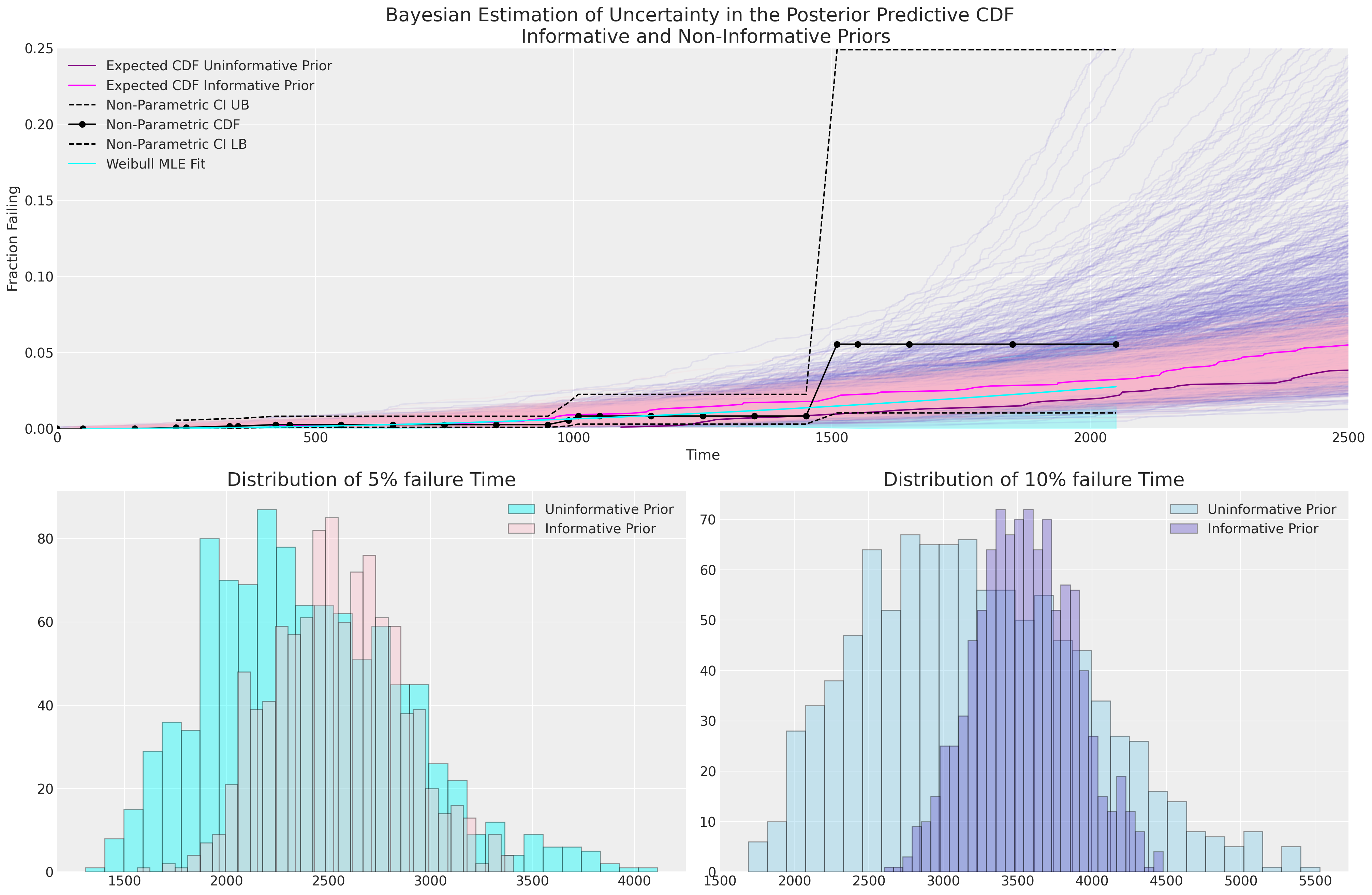
We can see here how the Bayesian uncertainty estimates driven by our deliberately vague priors encompasses more uncertainty than our MLE fit and the uninformative prior implies a wider predictive distribution for the 5% and 10% failure times. The Bayesian model with uninformative priors seems to do a better job of capturing the uncertainty in the non-parametric estimates of our CDF, but without more information it’s hard to tell which is the more appropriate model.
The concrete estimates of failure percentage over time of each model fit are especially crucial in a situation where we have sparse data. It is a meaningful sense check that we can consult with subject matter experts about how plausible the expectation and range for the 10% failure time is for their product.
Predicting the Number of Failures in an Interval#
Because our data on observed failures is extremely sparse, we have to be very careful about extrapolating beyond the observed range of time, but we can ask about the predictable number of failures in the lower tail of our cdf. This provides another view on this data which can be helpful for discussing with subject matters experts.
The Plugin Estimate#
Imagine we want to know how many bearings will fail between 150 and 600 hours based of service. We can calculate this based on the estimated CDF and number of new future bearings. We first calculate:
to establish a probability for the failure occurring in the interval and then a point prediction for the number of failures in the interval is given by risk_set*\(\hat{\rho}\).
mle_fit = weibull_min(c=2, scale=10_000)
rho = mle_fit.cdf(600) - mle_fit.cdf(150) / (1 - mle_fit.cdf(150))
print("Rho:", rho)
print("N at Risk:", 1700)
print("Expected Number Failing in between 150 and 600 hours:", 1700 * rho)
print("Lower Bound 95% PI :", binom(1700, rho).ppf(0.05))
print("Upper Bound 95% PI:", binom(1700, rho).ppf(0.95))
Rho: 0.0033685024546080927
N at Risk: 1700
Expected Number Failing in between 150 and 600 hours: 5.7264541728337575
Lower Bound 95% PI : 2.0
Upper Bound 95% PI: 10.0
Applying the Same Procedure on the Bayesian Posterior#
We’ll use the posterior predictive distribution of the uniformative model. We show here how to derive the uncertainty in the estimates of the 95% prediction interval for the number of failures in a time interval. As we saw above the MLE alternative to this procedure is to generate a predictive distribution from bootstrap sampling. The bootstrap procedure tends to agree with the plug-in procedure using the MLE estimates and lacks the flexibility of specifying prior information.
import xarray as xr

from xarray_einstats.stats import XrContinuousRV, XrDiscreteRV


def PI_failures(joint_draws, lp, up, n_at_risk):
    fit = XrContinuousRV(weibull_min, joint_draws["alpha"], scale=joint_draws["beta"])
    rho = fit.cdf(up) - fit.cdf(lp) / (1 - fit.cdf(lp))
    lub = XrDiscreteRV(binom, n_at_risk, rho).ppf([0.05, 0.95])
    lb, ub = lub.sel(quantile=0.05, drop=True), lub.sel(quantile=0.95, drop=True)
    point_prediction = n_at_risk * rho
    return xr.Dataset(
        {"rho": rho, "n_at_risk": n_at_risk, "lb": lb, "ub": ub, "expected": point_prediction}
    )


output_ds = PI_failures(joint_draws, 150, 600, 1700)
output_ds
<xarray.Dataset>
Dimensions:    (sample: 1000)
Coordinates:
  * sample     (sample) object MultiIndex
  * chain      (sample) int64 1 0 0 0 2 1 1 2 1 3 0 2 ... 1 3 2 3 0 1 3 3 0 1 2
  * draw       (sample) int64 776 334 531 469 19 675 ... 437 470 242 662 316 63
Data variables:
    rho        (sample) float64 0.0007735 0.004392 ... 0.001465 0.001462
    n_at_risk  int64 1700
    lb         (sample) float64 0.0 3.0 0.0 0.0 0.0 1.0 ... 0.0 1.0 0.0 0.0 0.0
    ub         (sample) float64 3.0 12.0 5.0 5.0 4.0 7.0 ... 5.0 7.0 6.0 5.0 5.0
expected (sample) float64 1.315 7.466 2.24 2.518 ... 2.835 2.491 2.486def cost_func(failures, power):
### Imagined cost function for failing item e.g. refunds required
return np.power(failures, power)
mosaic = """AAAA
BBCC"""
fig, axs = plt.subplot_mosaic(mosaic=mosaic, figsize=(20, 12))
axs = [axs[k] for k in axs.keys()]
ax = axs[0]
ax1 = axs[1]
ax2 = axs[2]
ax.scatter(
joint_draws["alpha"],
output_ds["expected"],
c=joint_draws["beta"],
cmap=cm.cool,
alpha=0.3,
label="Coloured by function of Beta values",
)
ax.legend()
ax.set_ylabel("Expected Failures")
ax.set_xlabel("Alpha")
ax.set_title(
"Posterior Predictive Expected Failure Count between 150-600 hours \nas a function of Weibull(alpha, beta)",
fontsize=20,
)
ax1.hist(
output_ds["lb"],
ec="black",
color="slateblue",
label="95% PI Lower Bound on Failure Count",
alpha=0.3,
)
ax1.axvline(output_ds["lb"].mean(), label="Expected 95% PI Lower Bound on Failure Count")
ax1.axvline(output_ds["ub"].mean(), label="Expected 95% PI Upper Bound on Failure Count")
ax1.hist(
output_ds["ub"],
ec="black",
color="cyan",
label="95% PI Upper Bound on Failure Count",
bins=20,
alpha=0.3,
)
ax1.hist(
output_ds["expected"], ec="black", color="pink", label="Expected Count of Failures", bins=20
)
ax1.set_title("Uncertainty in the Posterior Prediction Interval of Failure Counts", fontsize=20)
ax1.legend()
ax2.set_title("Expected Costs Distribution(s) \nbased on implied Failure counts", fontsize=20)
ax2.hist(
cost_func(output_ds["expected"], 2.3),
label="Cost(failures,2)",
color="royalblue",
alpha=0.3,
ec="black",
bins=20,
)
ax2.hist(
cost_func(output_ds["expected"], 2),
label="Cost(failures,2.3)",
color="red",
alpha=0.5,
ec="black",
bins=20,
)
ax2.set_xlabel("$ cost")
# ax2.set_xlim(-60, 0)
ax2.legend();
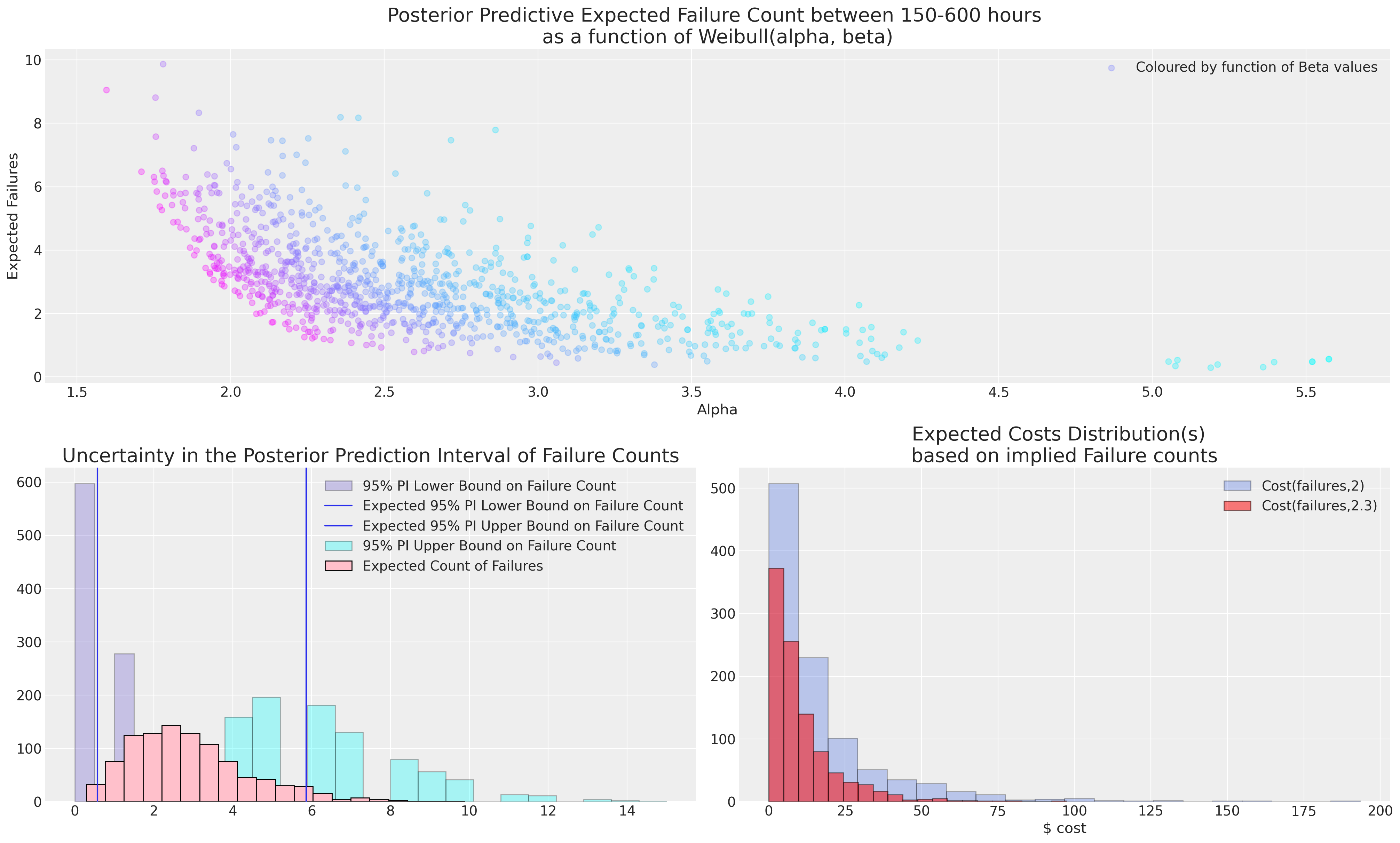
The choice of model in such cases is crucial. The decision about which failure profile is apt has to be informed by a subject matter expert because extrapolation from such sparse data is always risky. An understanding of the uncertainty is crucial if real costs attach to the failures and the subject matter expert is usually better placed to tell if you 2 or 7 failures can be plausibly expected within 600 hours of service.
Conclusion#
We’ve seen how to analyse and model reliability from both a frequentist and Bayesian perspective and compare against the non-parametric estimates. We’ve shown how prediction intervals can be derived for a number of key statistics by both a bootstrapping and a bayesian approach. We’ve seen approaches to calibrating these prediction intervals through re-sampling methods and informative prior specification. These views on the problem are complementary and the choice of technique which is appropriate should be driven by factors of the questions of interest, not some ideological commitment.
In particular we’ve seen how the MLE fits to our bearings data provide a decent first guess approach to establishing priors in the Bayesian analysis. We’ve also seen how subject matter expertise can be elicited by deriving key quantities from the implied models and subjecting these implications to scrutiny. The choice of Bayesian prediction interval is calibrated to our priors expectations, and where we have none - we can supply vague or non-informative priors. The implications of these priors can again be checked and analysed against an appropriate cost function.
References#
W.Q. Meeker, L.A. Escobar, and F.G Pascual. Statistical Methods for Reliability Data. Wiley, 2022.
Watermark#
%load_ext watermark
%watermark -n -u -v -iv -w -p pytensor,xarray_einstats
Last updated: Sun Jan 15 2023

Python implementation: CPython
Python version       : 3.10.8
IPython version      : 8.7.0

pytensor       : 2.8.10
xarray_einstats: 0.5.0.dev0

pandas    : 1.5.2
pymc      : 5.0.0
matplotlib: 3.6.2
xarray    : 2022.12.0
numpy     : 1.24.0
arviz     : 0.13.0

Watermark: 2.3.1
License notice#
All the notebooks in this example gallery are provided under the MIT License which allows modification, and redistribution for any use provided the copyright and license notices are preserved.
Citing PyMC examples#
To cite this notebook, use the DOI provided by Zenodo for the pymc-examples repository.
Important
Many notebooks are adapted from other sources: blogs, books… In such cases you should cite the original source as well.
Also remember to cite the relevant libraries used by your code.
Here is an citation template in bibtex:
@incollection{citekey,
  author    = "<notebook authors, see above>",
  title     = "<notebook title>",
  editor    = "PyMC Team",
  booktitle = "PyMC examples",
  doi       = "10.5281/zenodo.5654871"
}
which once rendered could look like: