


Factor analysis#
Factor analysis is a widely used probabilistic model for identifying low-rank structure in multivariate data as encoded in latent variables. It is very closely related to principal components analysis, and differs only in the prior distributions assumed for these latent variables. It is also a good example of a linear Gaussian model as it can be described entirely as a linear transformation of underlying Gaussian variates. For a high-level view of how factor analysis relates to other models, you can check out this diagram originally published by Ghahramani and Roweis.
Attention
This notebook uses libraries that are not PyMC dependencies and therefore need to be installed specifically to run this notebook. Open the dropdown below for extra guidance.
Extra dependencies install instructions
In order to run this notebook (either locally or on binder) you won’t only need a working PyMC installation with all optional dependencies, but also to install some extra dependencies. For advise on installing PyMC itself, please refer to Installation
You can install these dependencies with your preferred package manager, we provide as an example the pip and conda commands below.
$ pip install seaborn
Note that if you want (or need) to install the packages from inside the notebook instead of the command line, you can install the packages by running a variation of the pip command:
import sys
!{sys.executable} -m pip install seaborn
You should not run !pip install as it might install the package in a different
environment and not be available from the Jupyter notebook even if installed.
Another alternative is using conda instead:
$ conda install seaborn
when installing scientific python packages with conda, we recommend using conda forge
import arviz as az
import numpy as np
import pymc as pm
import pytensor.tensor as pt
import scipy as sp
import seaborn as sns
import xarray as xr

from matplotlib import pyplot as plt
from numpy.random import default_rng
from xarray_einstats import linalg
from xarray_einstats.stats import XrContinuousRV

print(f"Running on PyMC v{pm.__version__}")
Running on PyMC v5.28.0+58.gf58491a3
%config InlineBackend.figure_format = 'retina'
az.style.use("arviz-variat")

np.set_printoptions(precision=3, suppress=True)
RANDOM_SEED = 31415
rng = default_rng(RANDOM_SEED)
Simulated data generation#
To work through a few examples, we’ll first generate some data. The data will not follow the exact generative process assumed by the factor analysis model, as the latent variates will not be Gaussian. We’ll assume that we have an observed data set with \(N\) rows and \(d\) columns which are actually a noisy linear function of \(k_{true}\) latent variables.
n = 250
k_true = 4
d = 10
The next code cell generates the data via creating latent variable arrays M and linear transformation Q. Then, the matrix product \(QM\) is perturbed with additive Gaussian noise controlled by the variance parameter err_sd.
Because of the way we have generated the data, the covariance matrix expressing correlations between columns of \(Y\) will be equal to \(QQ^T\). The fundamental assumption of PCA and factor analysis is that \(QQ^T\) is not full rank. We can see hints of this if we plot the covariance matrix:
plt.figure(figsize=(4, 3))
sns.heatmap(np.corrcoef(Y));
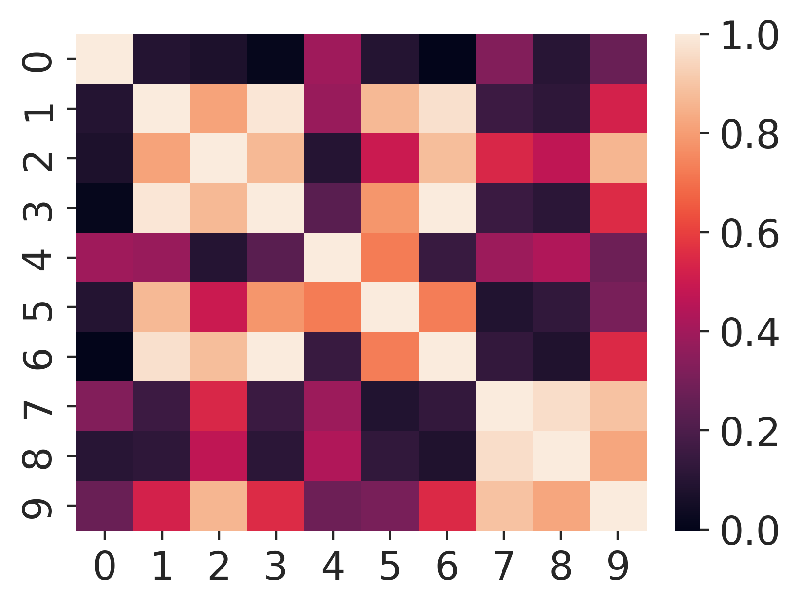
If you squint long enough, you may be able to glimpse a few places where distinct columns are likely linear functions of each other.
Model#
Probabilistic PCA (PPCA) and factor analysis (FA) are a common source of topics on PyMC Discourse. The posts linked below handle different aspects of the problem including:
Direct implementation#
The model for factor analysis is the probabilistic matrix factorization
\(X_{(d,n)}|W_{(d,k)}, F_{(k,n)} \sim \mathcal{N}(WF, \Psi)\)
with \(\Psi\) a diagonal matrix. Subscripts denote the dimensionality of the matrices. Probabilistic PCA is a variant that sets \(\Psi = \sigma^2 I\). A basic implementation (taken from this gist) is shown in the next cell. Unfortunately, it has undesirable properties for model fitting.
k = 2

coords = {"latent_columns": np.arange(k), "rows": np.arange(n), "observed_columns": np.arange(d)}

with pm.Model(coords=coords) as PPCA:
    W = pm.Normal("W", dims=("observed_columns", "latent_columns"))
    F = pm.Normal("F", dims=("latent_columns", "rows"))
    sigma = pm.HalfNormal("sigma", 1.0)
    X = pm.Normal("X", mu=W @ F, sigma=sigma, observed=Y, dims=("observed_columns", "rows"))

    trace = pm.sample(tune=2000, random_seed=rng)  # target_accept=0.9
Initializing NUTS using jitter+adapt_diag...
Multiprocess sampling (4 chains in 4 jobs)
NUTS: [W, F, sigma]
Sampling 4 chains for 2_000 tune and 1_000 draw iterations (8_000 + 4_000 draws total) took 12 seconds.
The rhat statistic is larger than 1.01 for some parameters. This indicates problems during sampling. See https://arxiv.org/abs/1903.08008 for details
The effective sample size per chain is smaller than 100 for some parameters.  A higher number is needed for reliable rhat and ess computation. See https://arxiv.org/abs/1903.08008 for details
At this point, there are already several warnings regarding failed convergence checks. We can see further problems in the trace plot below. This plot shows the path taken by each sampler chain for a single entry in the matrix \(W\) as well as the average evaluated over samples for each chain.
az.plot_trace(
    trace,
    var_names="W",
    coords={"observed_columns": 3, "latent_columns": 1},
    sample_dims=["draw"],
    figure_kwargs={"sharey": True},
);
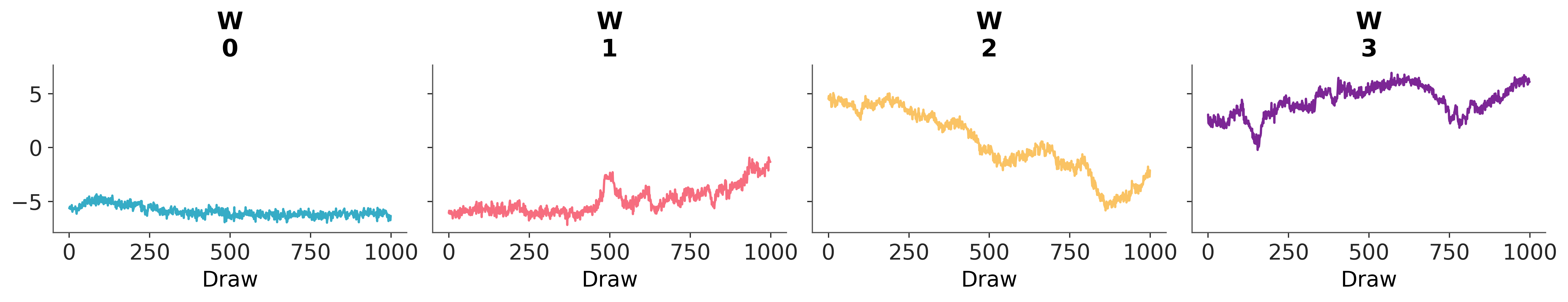
Each chain appears to have a different sample mean and we can also see that there is a great deal of autocorrelation across chains, manifest as long-range trends over sampling iterations.
One of the primary drawbacks for this model formulation is its lack of identifiability. With this model representation, only the product \(WF\) matters for the likelihood of \(X\), so \(P(X|W, F) = P(X|W\Omega, \Omega^{-1}F)\) for any invertible matrix \(\Omega\). While the priors on \(W\) and \(F\) constrain \(|\Omega|\) to be neither too large or too small, factors and loadings can still be rotated, reflected, and/or permuted without changing the model likelihood. Expect it to happen between runs of the sampler, or even for the parametrization to “drift” within run, and to produce the highly autocorrelated \(W\) traceplot above.
Alternative parametrization#
This can be fixed by constraining the form of W to be:
Lower triangular
Positive and increasing values along the diagonal
We can adapt expand_block_triangular to fill out a non-square matrix. This function mimics pm.expand_packed_triangular, but while the latter only works on packed versions of square matrices (i.e. \(d=k\) in our model, the former can also be used with nonsquare matrices.
def expand_packed_block_triangular(d, k, packed, diag=None, mtype="pytensor"):
    # like expand_packed_triangular, but with d > k.
    assert mtype in {"pytensor", "numpy"}
    assert d >= k

    def set_(M, i_, v_):
        if mtype == "pytensor":
            return pt.set_subtensor(M[i_], v_)
        M[i_] = v_
        return M

    out = pt.zeros((d, k), dtype=float) if mtype == "pytensor" else np.zeros((d, k), dtype=float)
    if diag is None:
        idxs = np.tril_indices(d, m=k)
        out = set_(out, idxs, packed)
    else:
        idxs = np.tril_indices(d, k=-1, m=k)
        out = set_(out, idxs, packed)
        idxs = (np.arange(k), np.arange(k))
        out = set_(out, idxs, diag)
    return out
We’ll also define another function which helps create a diagonal matrix with increasing entries along the main diagonal.
def makeW(d, k, dim_names):
    # make a W matrix adapted to the data shape
    n_od = int(k * d - k * (k - 1) / 2 - k)

    # trick: the cumulative sum of z will be positive increasing
    z = pm.HalfNormal("W_z", 1.0, dims="latent_columns")
    b = pm.Normal("W_b", 0.0, 1.0, shape=(n_od,), dims="packed_dim")
    L = expand_packed_block_triangular(d, k, b, pt.ones(k))
    W = pm.Deterministic("W", L @ pt.diag(pt.extra_ops.cumsum(z)), dims=dim_names)
    return W
With these modifications, we remake the model and run the MCMC sampler again.
with pm.Model(coords=coords) as PPCA_identified:
    W = makeW(d, k, ("observed_columns", "latent_columns"))
    F = pm.Normal("F", dims=("latent_columns", "rows"))
    sigma = pm.HalfNormal("sigma", 1.0)
    X = pm.Normal("X", mu=W @ F, sigma=sigma, observed=Y, dims=("observed_columns", "rows"))
    trace = pm.sample(tune=2000, random_seed=rng, target_accept=0.9)
Initializing NUTS using jitter+adapt_diag...
Multiprocess sampling (4 chains in 4 jobs)
NUTS: [W_z, W_b, F, sigma]
/home/osvaldo/anaconda3/envs/arviz_1/lib/python3.14/site-packages/pymc/step_methods/hmc/quadpotential.py:316: RuntimeWarning: overflow encountered in dot
  return 0.5 * np.dot(x, v_out)
Sampling 4 chains for 2_000 tune and 1_000 draw iterations (8_000 + 4_000 draws total) took 15 seconds.
The rhat statistic is larger than 1.01 for some parameters. This indicates problems during sampling. See https://arxiv.org/abs/1903.08008 for details
The effective sample size per chain is smaller than 100 for some parameters.  A higher number is needed for reliable rhat and ess computation. See https://arxiv.org/abs/1903.08008 for details
\(W\) (and \(F\)!) now have entries with identical posterior distributions as compared between sampler chains, although it’s apparent that some autocorrelation remains.
Because the \(k \times n\) parameters in F all need to be sampled, sampling can become quite expensive for very large n. In addition, the link between an observed data point \(X_i\) and an associated latent value \(F_i\) means that streaming inference with mini-batching cannot be performed.
This scalability problem can be addressed analytically by integrating \(F\) out of the model. By doing so, we postpone any calculation for individual values of \(F_i\) until later. Hence, this approach is often described as amortized inference. However, this fixes the prior on \(F\), allowing for less modeling flexibility. In keeping with \(F_{ij} \sim \mathcal{N}(0, I)\) we have:
\(X|WF \sim \mathcal{N}(WF, \sigma^2 I).\)
We can therefore write \(X\) as
\(X = WF + \sigma I \epsilon,\)
where \(\epsilon \sim \mathcal{N}(0, I)\). Fixing \(W\) but treating \(F\) and \(\epsilon\) as random variables, both \(\sim\mathcal{N}(0, I)\), we see that \(X\) is the sum of two multivariate normal variables, with means \(0\) and covariances \(WW^T\) and \(\sigma^2 I\), respectively. It follows that
\(X|W \sim \mathcal{N}(0, WW^T + \sigma^2 I )\).
with pm.Model(coords=coords) as PPCA_amortized:
    W = makeW(d, k, ("observed_columns", "latent_columns"))
    sigma = pm.HalfNormal("sigma", 1.0)
    cov = W @ W.T + sigma**2 * pt.eye(d)
    # MvNormal parametrizes covariance of columns, so transpose Y
    X = pm.MvNormal("X", 0.0, cov=cov, observed=Y.T, dims=("rows", "observed_columns"))
    trace_amortized = pm.sample(tune=30, draws=100, random_seed=rng)
Initializing NUTS using jitter+adapt_diag...
Multiprocess sampling (4 chains in 4 jobs)
NUTS: [W_z, W_b, sigma]
/home/osvaldo/anaconda3/envs/arviz_1/lib/python3.14/site-packages/pymc/step_methods/hmc/quadpotential.py:316: RuntimeWarning: overflow encountered in dot
  return 0.5 * np.dot(x, v_out)
Sampling 4 chains for 30 tune and 100 draw iterations (120 + 400 draws total) took 9 seconds.
The rhat statistic is larger than 1.01 for some parameters. This indicates problems during sampling. See https://arxiv.org/abs/1903.08008 for details
The effective sample size per chain is smaller than 100 for some parameters.  A higher number is needed for reliable rhat and ess computation. See https://arxiv.org/abs/1903.08008 for details
Unfortunately sampling of this model is very slow, presumably because calculating the logprob of the MvNormal requires inverting the covariance matrix. However, the explicit integration of \(F\) also enables batching the observations for faster computation of ADVI and FullRankADVI approximations.
coords["observed_columns2"] = coords["observed_columns"]
with pm.Model(coords=coords) as PPCA_amortized_batched:
    W = makeW(d, k, ("observed_columns", "latent_columns"))
    Y_mb = pm.Minibatch(
        Y.T, batch_size=50
    )  # MvNormal parametrizes covariance of columns, so transpose Y
    sigma = pm.HalfNormal("sigma", 1.0)
    cov = W @ W.T + sigma**2 * pt.eye(d)
    X = pm.MvNormal("X", 0.0, cov=cov, observed=Y_mb)
    trace_vi = pm.fit(n=50000, method="fullrank_advi", obj_n_mc=1).sample()
/home/osvaldo/anaconda3/envs/arviz_1/lib/python3.14/site-packages/pymc/model/core.py:1256: UserWarning: total_size not provided for observed variable `X` that uses pm.Minibatch
  warnings.warn(
Finished [100%]: Average Loss = 1,758.4
Results#
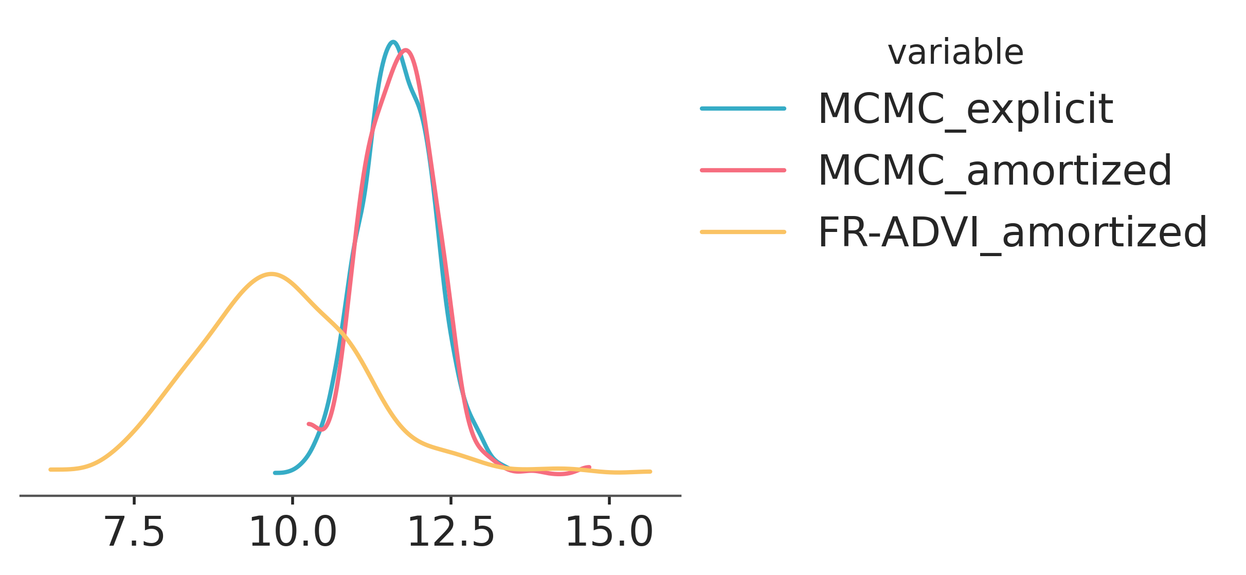
When we compare the posteriors calculated using MCMC and VI, we find that (for at least this specific parameter we are looking at) the two distributions are close, but they do differ in their mean. The two MCMC posteriors agree with each other quite well with each other and the ADVI estimate is not far off.
col_selection = dict(observed_columns=3, latent_columns=1)

dt = az.from_dict(
    {
        "posterior": {
            "MCMC_explicit": trace.posterior["W"].sel(**col_selection),
            "MCMC_amortized": trace_amortized.posterior["W"].sel(**col_selection),
            "FR-ADVI_amortized": trace_vi.posterior["W"].sel(**col_selection),
        }
    }
)

pc = az.plot_dist(
    dt,
    cols=None,
    aes={"color": ["__variable__"]},
    visuals={
        "title": False,
        "point_estimate_text": False,
        "point_estimate": False,
        "credible_interval": False,
    },
)
pc.add_legend("__variable__")
Post-hoc identification of F#
The matrix \(F\) is typically of interest for factor analysis, and is often used as a feature matrix for dimensionality reduction. However, \(F\) has been marginalized away in order to make fitting the model easier; and now we need it back. Transforming
\(X|WF \sim \mathcal{N}(WF, \sigma^2)\)
into
\((W^TW)^{-1}W^T X|W,F \sim \mathcal{N}(F, \sigma^2(W^TW)^{-1})\)
we have represented \(F\) as the mean of a multivariate normal distribution with a known covariance matrix. Using the prior \( F \sim \mathcal{N}(0, I) \) and updating according to the expression for the conjugate prior, we find
\( F | X, W \sim \mathcal{N}(\mu_F, \Sigma_F) \),
where
\(\mu_F = \left(I + \sigma^{-2} W^T W\right)^{-1} \sigma^{-2} W^T X\)
\(\Sigma_F = \left(I + \sigma^{-2} W^T W\right)^{-1}\)
For each value of \(W\) and \(X\) found in the trace, we now draw a sample from this distribution.
# configure xarray-einstats
def get_default_dims(dims, dims2):
    proposed_dims = [dim for dim in dims if dim not in {"chain", "draw"}]
    assert len(proposed_dims) == 2
    if dims2 is None:
        return proposed_dims


linalg.get_default_dims = get_default_dims
post = trace_vi.posterior
obs = trace.observed_data

WW = linalg.matmul(
    post["W"], post["W"], dims=("latent_columns", "observed_columns", "latent_columns")
)

# Constructing an identity matrix following https://einstats.python.arviz.org/en/latest/tutorials/np_linalg_tutorial_port.html
I = xr.zeros_like(WW)
idx = xr.DataArray(WW.coords["latent_columns"])
I.loc[{"latent_columns": idx, "latent_columns2": idx}] = 1
Sigma_F = linalg.inv(I + post["sigma"] ** (-2) * WW)
X_transform = linalg.matmul(
    Sigma_F,
    post["sigma"] ** (-2) * post["W"],
    dims=("latent_columns2", "latent_columns", "observed_columns"),
)
mu_F = xr.dot(X_transform, obs["X"], dims="observed_columns").rename(
    latent_columns2="latent_columns"
)
Sigma_chol = linalg.cholesky(Sigma_F)
norm_dist = XrContinuousRV(sp.stats.norm, xr.zeros_like(mu_F))  # the zeros_like defines the shape
F_sampled = mu_F + linalg.matmul(
    post["sigma"] * Sigma_F,
    norm_dist.rvs(),
    dims=(("latent_columns", "latent_columns2"), ("latent_columns", "rows")),
)
Comparison to original data#
To check how well our model has captured the original data, we will test how well we can reconstruct it from the sampled \(W\) and \(F\) matrices. For each element of \(Y\) we plot the mean and standard deviation of \(X = W F\), which is the reconstructed value based on our model.
X_sampled_amortized = linalg.matmul(
    post["W"],
    F_sampled,
    dims=("observed_columns", "latent_columns", "rows"),
)
reconstruction_mean = X_sampled_amortized.mean(dim=("chain", "draw")).values
reconstruction_sd = X_sampled_amortized.std(dim=("chain", "draw")).values
plt.errorbar(
    Y.ravel(),
    reconstruction_mean.ravel(),
    yerr=reconstruction_sd.ravel(),
    marker=".",
    ls="none",
    alpha=0.3,
)

slope, intercept, r_value, p_value, std_err = sp.stats.linregress(
    Y.ravel(), reconstruction_mean.ravel()
)
plt.plot(
    [Y.min(), Y.max()],
    np.array([Y.min(), Y.max()]) * slope + intercept,
    "k--",
    label=f"Linear regression for the mean, R²={r_value**2:.2f}",
)
plt.plot([Y.min(), Y.max()], [Y.min(), Y.max()], "k:", label="Perfect reconstruction")

plt.xlabel("Elements of Y")
plt.ylabel("Model reconstruction")
plt.legend(loc="upper left");
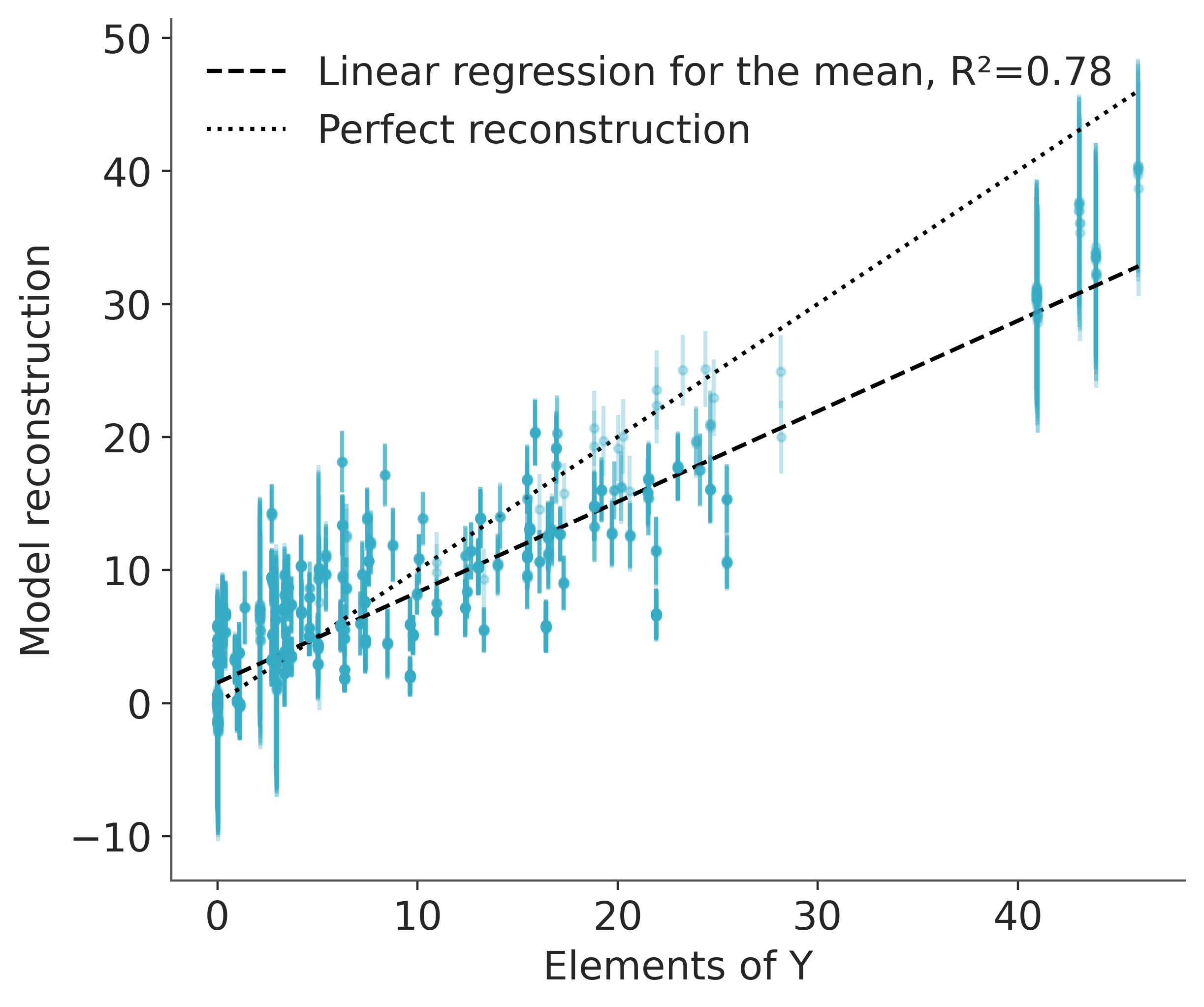
We find that our model does a decent job of capturing the variation in the original data, despite only using two latent factors instead of the actual four.
Watermark#
%load_ext watermark
%watermark -n -u -v -iv -w
Last updated: Sat, 25 Apr 2026

Python implementation: CPython
Python version       : 3.14.4
IPython version      : 9.12.0

arviz          : 1.1.0
matplotlib     : 3.10.8
numpy          : 2.4.4
pymc           : 5.28.0+58.gf58491a3
pytensor       : 2.38.0+133.g80cc113b5
scipy          : 1.17.1
seaborn        : 0.13.2
xarray         : 2026.4.0
xarray_einstats: 0.10.0

Watermark: 2.6.0
License notice#
All the notebooks in this example gallery are provided under the MIT License which allows modification, and redistribution for any use provided the copyright and license notices are preserved.
Citing PyMC examples#
To cite this notebook, use the DOI provided by Zenodo for the pymc-examples repository.
Important
Many notebooks are adapted from other sources: blogs, books… In such cases you should cite the original source as well.
Also remember to cite the relevant libraries used by your code.
Here is an citation template in bibtex:
@incollection{citekey,
  author    = "<notebook authors, see above>",
  title     = "<notebook title>",
  editor    = "PyMC Team",
  booktitle = "PyMC examples",
  doi       = "10.5281/zenodo.5654871"
}
which once rendered could look like: