GLM: Mini-batch ADVI on hierarchical regression model

Unlike Gaussian mixture models, (hierarchical) regression models have independent variables. These variables affect the likelihood function, but are not random variables. When using mini-batch, we should take care of that.

%env PYTENSOR_FLAGS=device=cpu, floatX=float32, warn_float64=ignore

import os

import arviz as az
import matplotlib.pyplot as plt
import numpy as np
import pandas as pd
import pymc as pm
import pytensor
import pytensor.tensor as pt
import seaborn as sns

from scipy import stats

print(f"Running on PyMC v{pm.__version__}")

env: PYTENSOR_FLAGS=device=cpu, floatX=float32, warn_float64=ignore
Running on PyMC v5.0.1

%config InlineBackend.figure_format = 'retina'
RANDOM_SEED = 8927
rng = np.random.default_rng(RANDOM_SEED)
az.style.use("arviz-darkgrid")

try:
    data = pd.read_csv(os.path.join("..", "data", "radon.csv"))
except FileNotFoundError:
    data = pd.read_csv(pm.get_data("radon.csv"))

data

	Unnamed: 0	idnum	state	state2	stfips	zip	region	typebldg	floor	room	...	pcterr	adjwt	dupflag	zipflag	cntyfips	county	fips	Uppm	county_code	log_radon
0	0	5081.0	MN	MN	27.0	55735	5.0	1.0	1.0	3.0	...	9.7	1146.499190	1.0	0.0	1.0	AITKIN	27001.0	0.502054	0	0.832909
1	1	5082.0	MN	MN	27.0	55748	5.0	1.0	0.0	4.0	...	14.5	471.366223	0.0	0.0	1.0	AITKIN	27001.0	0.502054	0	0.832909
2	2	5083.0	MN	MN	27.0	55748	5.0	1.0	0.0	4.0	...	9.6	433.316718	0.0	0.0	1.0	AITKIN	27001.0	0.502054	0	1.098612
3	3	5084.0	MN	MN	27.0	56469	5.0	1.0	0.0	4.0	...	24.3	461.623670	0.0	0.0	1.0	AITKIN	27001.0	0.502054	0	0.095310
4	4	5085.0	MN	MN	27.0	55011	3.0	1.0	0.0	4.0	...	13.8	433.316718	0.0	0.0	3.0	ANOKA	27003.0	0.428565	1	1.163151
...	...	...	...	...	...	...	...	...	...	...	...	...	...	...	...	...	...	...	...	...	...
914	914	5995.0	MN	MN	27.0	55363	5.0	1.0	0.0	4.0	...	4.5	1146.499190	0.0	0.0	171.0	WRIGHT	27171.0	0.913909	83	1.871802
915	915	5996.0	MN	MN	27.0	55376	5.0	1.0	0.0	7.0	...	8.3	1105.956867	0.0	0.0	171.0	WRIGHT	27171.0	0.913909	83	1.526056
916	916	5997.0	MN	MN	27.0	55376	5.0	1.0	0.0	4.0	...	5.2	1214.922779	0.0	0.0	171.0	WRIGHT	27171.0	0.913909	83	1.629241
917	917	5998.0	MN	MN	27.0	56297	5.0	1.0	0.0	4.0	...	9.6	1177.377355	0.0	0.0	173.0	YELLOW MEDICINE	27173.0	1.426590	84	1.335001
918	918	5999.0	MN	MN	27.0	56297	5.0	1.0	0.0	4.0	...	8.0	1214.922779	0.0	0.0	173.0	YELLOW MEDICINE	27173.0	1.426590	84	1.098612

919 rows × 30 columns

county_idx = data["county_code"].values
floor_idx = data["floor"].values
log_radon_idx = data["log_radon"].values

coords = {"counties": data.county.unique()}

Here, log_radon_idx_t is a dependent variable, while floor_idx_t and county_idx_t determine the independent variable.

log_radon_idx_t = pm.Minibatch(log_radon_idx, batch_size=100)
floor_idx_t = pm.Minibatch(floor_idx, batch_size=100)
county_idx_t = pm.Minibatch(county_idx, batch_size=100)

with pm.Model(coords=coords) as hierarchical_model:
    # Hyperpriors for group nodes
    mu_a = pm.Normal("mu_alpha", mu=0.0, sigma=100**2)
    sigma_a = pm.Uniform("sigma_alpha", lower=0, upper=100)
    mu_b = pm.Normal("mu_beta", mu=0.0, sigma=100**2)
    sigma_b = pm.Uniform("sigma_beta", lower=0, upper=100)

Intercept for each county, distributed around group mean mu_a. Above we just set mu and sd to a fixed value while here we plug in a common group distribution for all a and b (which are vectors with the same length as the number of unique counties in our example).

with hierarchical_model:
    a = pm.Normal("alpha", mu=mu_a, sigma=sigma_a, dims="counties")
    # Intercept for each county, distributed around group mean mu_a
    b = pm.Normal("beta", mu=mu_b, sigma=sigma_b, dims="counties")

Model prediction of radon level a[county_idx] translates to a[0, 0, 0, 1, 1, ...], we thus link multiple household measures of a county to its coefficients.

with hierarchical_model:
    radon_est = a[county_idx_t] + b[county_idx_t] * floor_idx_t

Finally, we specify the likelihood:

with hierarchical_model:
    # Model error
    eps = pm.Uniform("eps", lower=0, upper=100)

    # Data likelihood
    radon_like = pm.Normal(
        "radon_like", mu=radon_est, sigma=eps, observed=log_radon_idx_t, total_size=len(data)
    )

Random variables radon_like, associated with log_radon_idx_t, should be given to the function for ADVI to denote that as observations in the likelihood term.

On the other hand, minibatches should include the three variables above.

Then, run ADVI with mini-batch.

with hierarchical_model:
    approx = pm.fit(100_000, callbacks=[pm.callbacks.CheckParametersConvergence(tolerance=1e-4)])

idata_advi = approx.sample(500)

/home/fonnesbeck/mambaforge/envs/pie/lib/python3.9/site-packages/pymc/logprob/joint_logprob.py:167: UserWarning: Found a random variable that was neither among the observations nor the conditioned variables: [integers_rv{0, (0, 0), int64, False}.0, integers_rv{0, (0, 0), int64, False}.out]
  warnings.warn(
/home/fonnesbeck/mambaforge/envs/pie/lib/python3.9/site-packages/pymc/logprob/joint_logprob.py:167: UserWarning: Found a random variable that was neither among the observations nor the conditioned variables: [integers_rv{0, (0, 0), int64, False}.0, integers_rv{0, (0, 0), int64, False}.out]
  warnings.warn(
/home/fonnesbeck/mambaforge/envs/pie/lib/python3.9/site-packages/pymc/logprob/joint_logprob.py:167: UserWarning: Found a random variable that was neither among the observations nor the conditioned variables: [integers_rv{0, (0, 0), int64, False}.0, integers_rv{0, (0, 0), int64, False}.out]
  warnings.warn(
/home/fonnesbeck/mambaforge/envs/pie/lib/python3.9/site-packages/pymc/logprob/joint_logprob.py:167: UserWarning: Found a random variable that was neither among the observations nor the conditioned variables: [integers_rv{0, (0, 0), int64, False}.0, integers_rv{0, (0, 0), int64, False}.out]
  warnings.warn(

11.50% [11499/100000 00:03<00:27 Average Loss = 263.87]

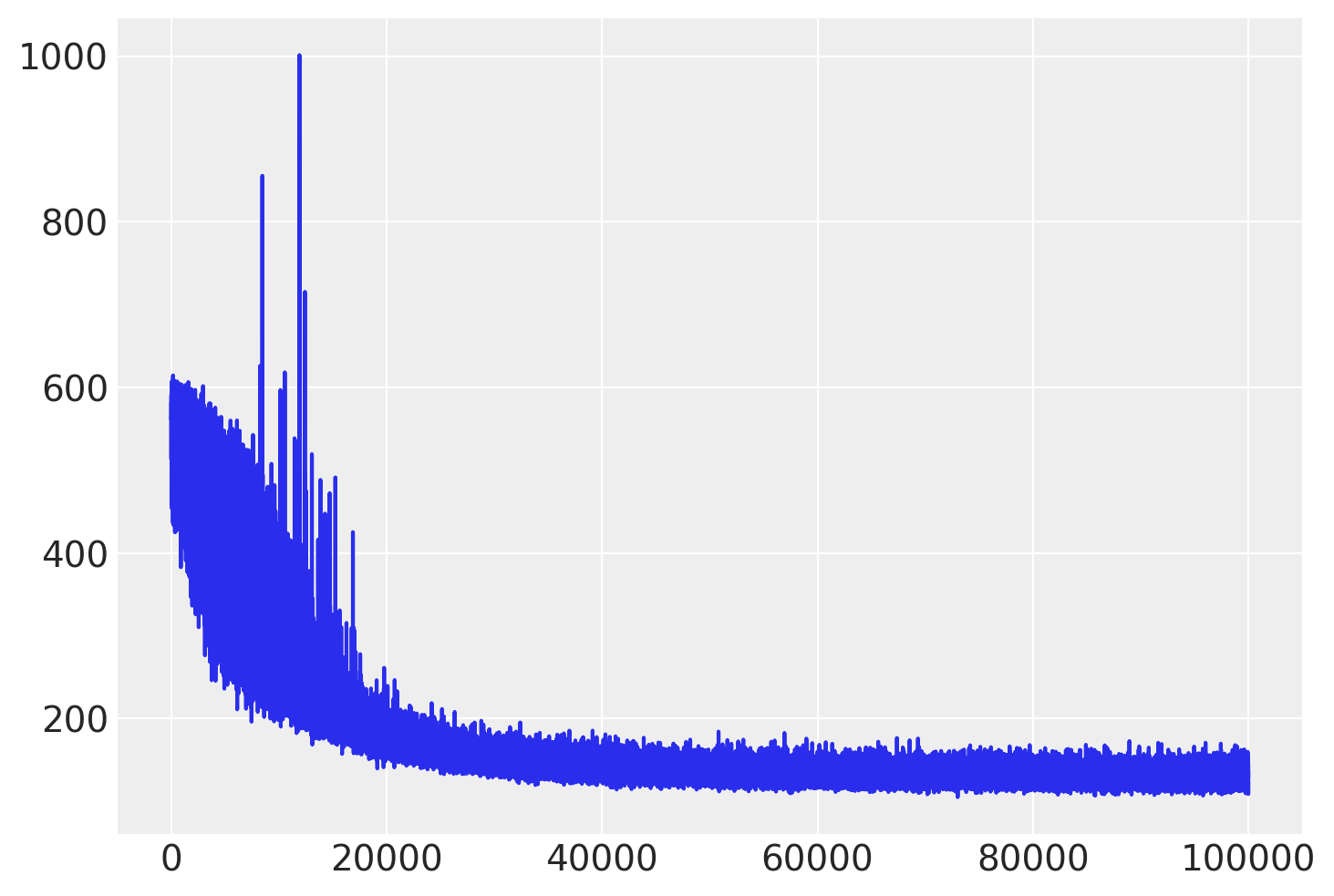
Check the trace of ELBO and compare the result with MCMC.

plt.plot(approx.hist);

We can extract the covariance matrix from the mean field approximation and use it as the scaling matrix for the NUTS algorithm.

scaling = approx.cov.eval()

Also, we can generate samples (one for each chain) to use as the starting points for the sampler.

n_chains = 4
sample = approx.sample(return_inferencedata=False, size=n_chains)
start_dict = list(sample[i] for i in range(n_chains))

# Inference button (TM)!
with pm.Model(coords=coords):
    mu_a = pm.Normal("mu_alpha", mu=0.0, sigma=100**2)
    sigma_a = pm.Uniform("sigma_alpha", lower=0, upper=100)
    mu_b = pm.Normal("mu_beta", mu=0.0, sigma=100**2)
    sigma_b = pm.Uniform("sigma_beta", lower=0, upper=100)

    a = pm.Normal("alpha", mu=mu_a, sigma=sigma_a, dims="counties")
    b = pm.Normal("beta", mu=mu_b, sigma=sigma_b, dims="counties")

    # Model error
    eps = pm.Uniform("eps", lower=0, upper=100)

    radon_est = a[county_idx] + b[county_idx] * floor_idx

    radon_like = pm.Normal("radon_like", mu=radon_est, sigma=eps, observed=log_radon_idx)

    # essentially, this is what init='advi' does
    step = pm.NUTS(scaling=scaling, is_cov=True)
    hierarchical_trace = pm.sample(draws=2000, step=step, chains=n_chains, initvals=start_dict)

Multiprocess sampling (4 chains in 4 jobs)
NUTS: [mu_alpha, sigma_alpha, mu_beta, sigma_beta, alpha, beta, eps]

100.00% [8000/8000 08:57<00:00 Sampling 4 chains, 0 divergences]

Sampling 4 chains for 1_000 tune and 1_000 draw iterations (4_000 + 4_000 draws total) took 538 seconds.

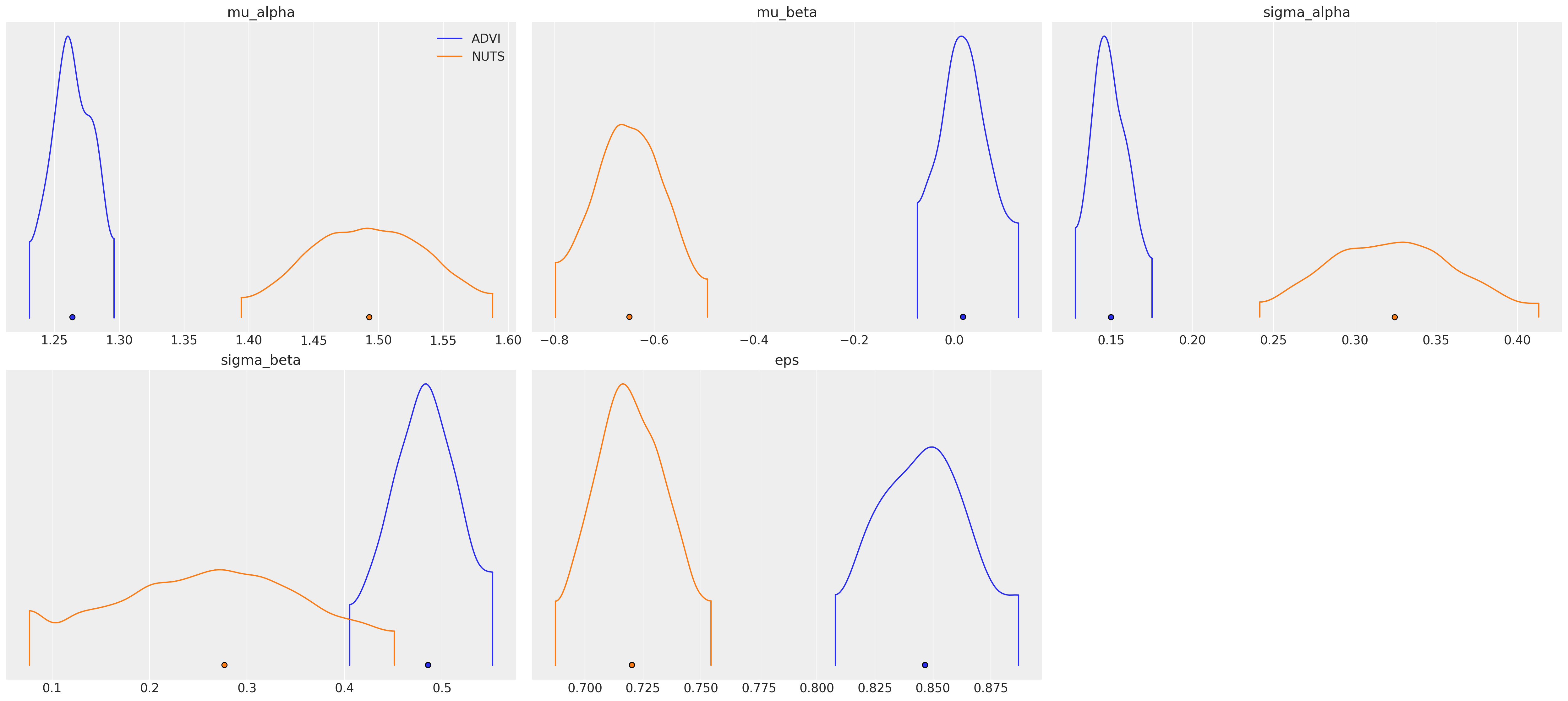
az.plot_density(
    data=[idata_advi, hierarchical_trace],
    var_names=["~alpha", "~beta"],
    data_labels=["ADVI", "NUTS"],
);

Watermark

%load_ext watermark
%watermark -n -u -v -iv -w -p xarray

Last updated: Thu Sep 23 2021

Python implementation: CPython
Python version       : 3.8.10
IPython version      : 7.25.0

xarray: 0.17.0

numpy     : 1.21.0
seaborn   : 0.11.1
pandas    : 1.2.1
matplotlib: 3.3.4
theano    : 1.1.2
pymc3     : 3.11.2
scipy     : 1.7.1
arviz     : 0.11.2

Watermark: 2.2.0

License notice

All the notebooks in this example gallery are provided under the MIT License which allows modification, and redistribution for any use provided the copyright and license notices are preserved.

Citing PyMC examples

To cite this notebook, use the DOI provided by Zenodo for the pymc-examples repository.

Important

Many notebooks are adapted from other sources: blogs, books… In such cases you should cite the original source as well.

Also remember to cite the relevant libraries used by your code.

Here is an citation template in bibtex:

@incollection{citekey,
  author    = "<notebook authors, see above>",
  title     = "<notebook title>",
  editor    = "PyMC Team",
  booktitle = "PyMC examples",
  doi       = "10.5281/zenodo.5654871"
}

which once rendered could look like: