Lasso regression with block updating#

%matplotlib inline
import arviz as az
import matplotlib.pyplot as plt
import numpy as np
import pymc as pm

print(f"Running on PyMC v{pm.__version__}")

Running on PyMC v4.0.0b2

RANDOM_SEED = 8927
rng = np.random.default_rng(RANDOM_SEED)
az.style.use("arviz-darkgrid")

Sometimes, it is very useful to update a set of parameters together. For example, variables that are highly correlated are often good to update together. In PyMC block updating is simple. This will be demonstrated using the parameter step of pymc.sample.

Here we have a LASSO regression model where the two coefficients are strongly correlated. Normally, we would define the coefficient parameters as a single random variable, but here we define them separately to show how to do block updates.

First we generate some fake data.

x = rng.standard_normal(size=(3, 30))
x1 = x[0] + 4
x2 = x[1] + 4
noise = x[2]
y_obs = x1 * 0.2 + x2 * 0.3 + noise

Then define the random variables.

lam = 3000

with pm.Model() as model:
    sigma = pm.Exponential("sigma", 1)
    tau = pm.Uniform("tau", 0, 1)
    b = lam * tau
    beta1 = pm.Laplace("beta1", 0, b)
    beta2 = pm.Laplace("beta2", 0, b)

    mu = x1 * beta1 + x2 * beta2

    y = pm.Normal("y", mu=mu, sigma=sigma, observed=y_obs)

For most samplers, including pymc.Metropolis and pymc.HamiltonianMC, simply pass a list of variables to sample as a block. This works with both scalar and array parameters.

with model:
    step1 = pm.Metropolis([beta1, beta2])

    step2 = pm.Slice([sigma, tau])

    idata = pm.sample(draws=10000, step=[step1, step2])

Multiprocess sampling (4 chains in 4 jobs)
CompoundStep
>CompoundStep
>>Metropolis: [beta1]
>>Metropolis: [beta2]
>CompoundStep
>>Slice: [sigma]
>>Slice: [tau]

100.00% [44000/44000 00:36<00:00 Sampling 4 chains, 0 divergences]

Sampling 4 chains for 1_000 tune and 10_000 draw iterations (4_000 + 40_000 draws total) took 37 seconds.
The number of effective samples is smaller than 10% for some parameters.

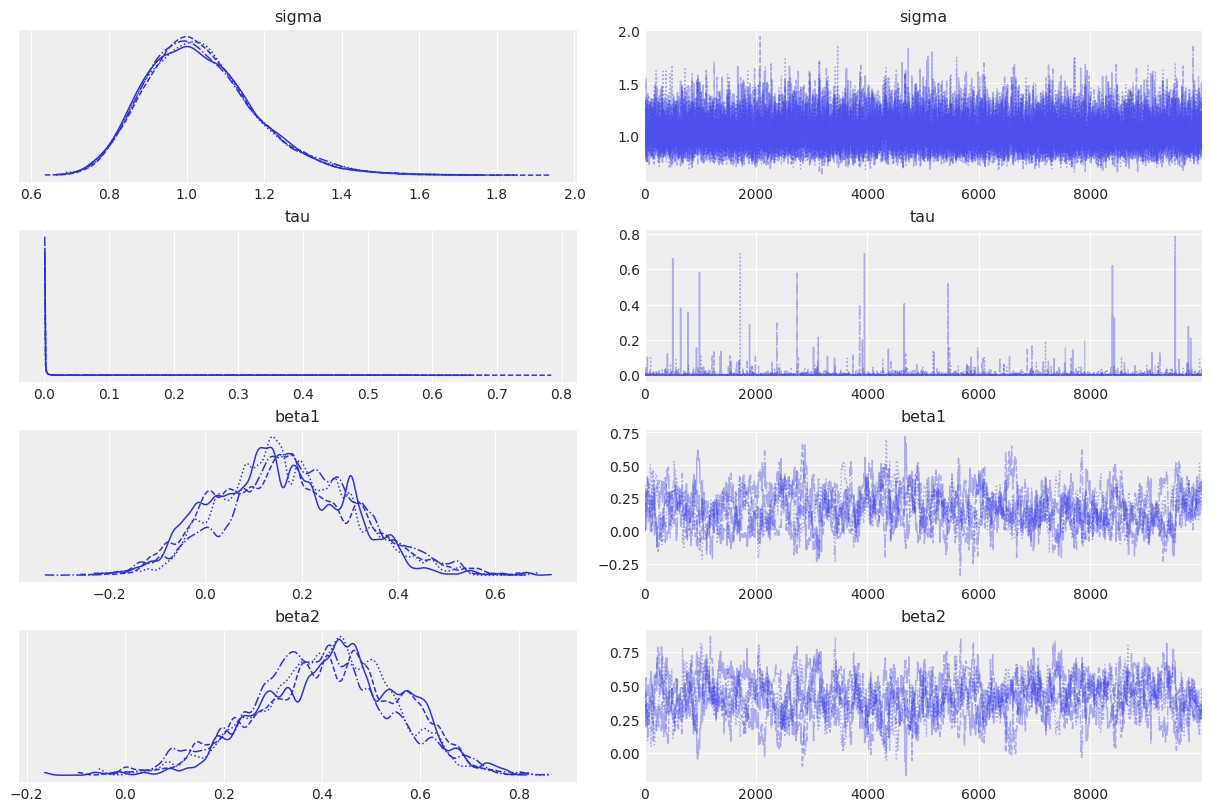
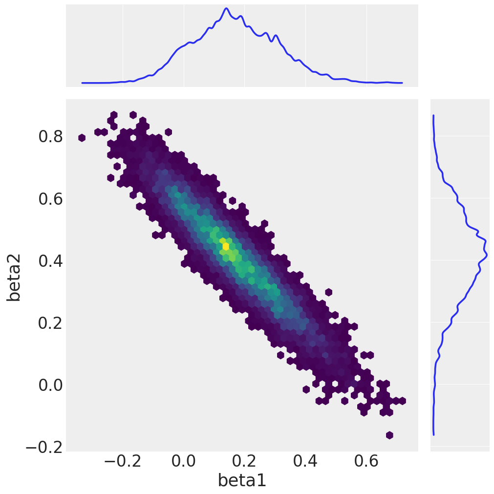
We conclude by plotting the sampled marginals and the joint distribution of beta1 and beta2.

az.plot_trace(idata);

../_images/0e88fba95c22b32165ed71adbc218847af2815a3f51302229e16df872cda552a.png

az.plot_pair(
    idata,
    var_names=["beta1", "beta2"],
    kind="hexbin",
    marginals=True,
    figsize=(10, 10),
    gridsize=50,
)

array([[<AxesSubplot:>, None],
       [<AxesSubplot:xlabel='beta1', ylabel='beta2'>, <AxesSubplot:>]],
      dtype=object)

../_images/2bc755fd8bf0a29be0c099502d53d2097de89708e8fd4c792426392f28773e1f.png

Authors#

Authored by Chris Fonnesbeck in Dec, 2020
Updated by Raul Maldonado in Jan, 2021
Updated by Raul Maldonado in Mar, 2021
Reexecuted by Thomas Wiecki and Michael Osthege with PyMC v4 in Jan, 2022 (pymc-examples#264)
Updated by Lorenzo Toniazzi in Feb, 2022 (pymc-examples#279)

Watermark#

%load_ext watermark
%watermark -n -u -v -iv -w -p pytensor,aeppl,xarray

Last updated: Thu Mar 03 2022

Python implementation: CPython
Python version       : 3.9.10
IPython version      : 8.0.1

pytensor: 2.3.2
aeppl : 0.0.18
xarray: 2022.3.0

pymc      : 4.0.0b2
matplotlib: 3.5.1
numpy     : 1.21.5
arviz     : 0.11.4

Watermark: 2.3.0

License notice#

All the notebooks in this example gallery are provided under the MIT License which allows modification, and redistribution for any use provided the copyright and license notices are preserved.

Citing PyMC examples#

To cite this notebook, use the DOI provided by Zenodo for the pymc-examples repository.

Important

Many notebooks are adapted from other sources: blogs, books… In such cases you should cite the original source as well.

Also remember to cite the relevant libraries used by your code.

Here is an citation template in bibtex:

@incollection{citekey,
  author    = "<notebook authors, see above>",
  title     = "<notebook title>",
  editor    = "PyMC Team",
  booktitle = "PyMC examples",
  doi       = "10.5281/zenodo.5654871"
}

which once rendered could look like:

Categories

Tags