Dirichlet mixtures of multinomials

This example notebook demonstrates the use of a Dirichlet mixture of multinomials (a.k.a Dirichlet-multinomial or DM) to model categorical count data. Models like this one are important in a variety of areas, including natural language processing, ecology, bioinformatics, and more.

The Dirichlet-multinomial can be understood as draws from a Multinomial distribution where each sample has a slightly different probability vector, which is itself drawn from a common Dirichlet distribution. This contrasts with the Multinomial distribution, which assumes that all observations arise from a single fixed probability vector. This enables the Dirichlet-multinomial to accommodate more variable (a.k.a, over-dispersed) count data than the Multinomial.

Other examples of over-dispersed count distributions are the Beta-binomial (which can be thought of as a special case of the DM) or the Negative binomial distributions.

The DM is also an example of marginalizing a mixture distribution over its latent parameters. This notebook will demonstrate the performance benefits that come from taking that approach.

import arviz as az
import matplotlib.pyplot as plt
import numpy as np
import pymc as pm
import scipy as sp

print(f"Running on PyMC v{pm.__version__}")

Running on PyMC v5.9.0

%config InlineBackend.figure_format = 'retina'
RANDOM_SEED = 8927
rng = np.random.default_rng(RANDOM_SEED)
az.style.use("arviz-darkgrid")

Simulation data

Let us simulate some over-dispersed, categorical count data for this example.

Here we are simulating from the DM distribution itself, so it is perhaps tautological to fit that model, but rest assured that data like these really do appear in the counts of different:

1. words in text corpuses [],

2. types of RNA molecules in a cell [],

3. items purchased by shoppers [].

Here we will discuss a community ecology example, pretending that we have observed counts of \(k=5\) different tree species in \(n=10\) different forests.

Our simulation will produce a two-dimensional matrix of integers (counts) where each row, (zero-)indexed by \(i \in (0...n-1)\), is an observation (different forest), and each column \(j \in (0...k-1)\) is a category (tree species). We’ll parameterize this distribution with three things:

• \(\mathrm{frac}\) : the expected fraction of each species, a \(k\)-dimensional vector on the simplex (i.e. sums-to-one)

• \(\mathrm{total\_count}\) : the total number of items tallied in each observation,

• \(\mathrm{conc}\) : the concentration, controlling the overdispersion of our data, where larger values result in our distribution more closely approximating the multinomial.

Here, and throughout this notebook, we’ve used a convenient reparameterization of the Dirichlet distribution from one to two parameters, \(\alpha=\mathrm{conc} \times \mathrm{frac}\), as this fits our desired interpretation.

Each observation from the DM is simulated by:

1. first obtaining a value on the \(k\)-simplex simulated as \(p_i \sim \mathrm{Dirichlet}(\alpha=\mathrm{conc} \times \mathrm{frac})\),

2. and then simulating \(\mathrm{counts}_i \sim \mathrm{Multinomial}(\mathrm{total\_count}, p_i)\).

Notice that each observation gets its own latent parameter \(p_i\), simulated independently from a common Dirichlet distribution.

true_conc = 6.0
true_frac = np.array([0.45, 0.30, 0.15, 0.09, 0.01])
trees = ["pine", "oak", "ebony", "rosewood", "mahogany"]  # Tree species observed
# fmt: off
forests = [  # Forests observed
    "sunderbans", "amazon", "arashiyama", "trossachs", "valdivian",
    "bosc de poblet", "font groga", "monteverde", "primorye", "daintree",
]
# fmt: on
k = len(trees)
n = len(forests)
total_count = 50

true_p = sp.stats.dirichlet(true_conc * true_frac).rvs(size=n, random_state=rng)
observed_counts = np.vstack(
    [sp.stats.multinomial(n=total_count, p=p_i).rvs(random_state=rng) for p_i in true_p]
)

observed_counts

array([[21,  9, 11,  6,  3],
       [36,  7,  6,  1,  0],
       [ 8, 31,  1, 10,  0],
       [25,  4, 17,  4,  0],
       [43,  6,  1,  0,  0],
       [28, 10, 12,  0,  0],
       [21, 16, 10,  3,  0],
       [16, 32,  2,  0,  0],
       [45,  4,  1,  0,  0],
       [35,  5,  2,  8,  0]])

Multinomial model

The first model that we will fit to these data is a plain multinomial model, where the only parameter is the expected fraction of each category, \(\mathrm{frac}\), which we will give a Dirichlet prior. While the uniform prior (\(\alpha_j=1\) for each \(j\)) works well, if we have independent beliefs about the fraction of each tree, we could encode this into our prior, e.g. increasing the value of \(\alpha_j\) where we expect a higher fraction of species-\(j\).

coords = {"tree": trees, "forest": forests}
with pm.Model(coords=coords) as model_multinomial:
    frac = pm.Dirichlet("frac", a=np.ones(k), dims="tree")
    counts = pm.Multinomial(
        "counts", n=total_count, p=frac, observed=observed_counts, dims=("forest", "tree")
    )

pm.model_to_graphviz(model_multinomial)

with model_multinomial:
    trace_multinomial = pm.sample(chains=4)

Auto-assigning NUTS sampler...
Initializing NUTS using jitter+adapt_diag...
Multiprocess sampling (4 chains in 4 jobs)
NUTS: [frac]

100.00% [8000/8000 00:02<00:00 Sampling 4 chains, 0 divergences]

Sampling 4 chains for 1_000 tune and 1_000 draw iterations (4_000 + 4_000 draws total) took 2 seconds.

az.plot_trace(data=trace_multinomial, var_names=["frac"]);

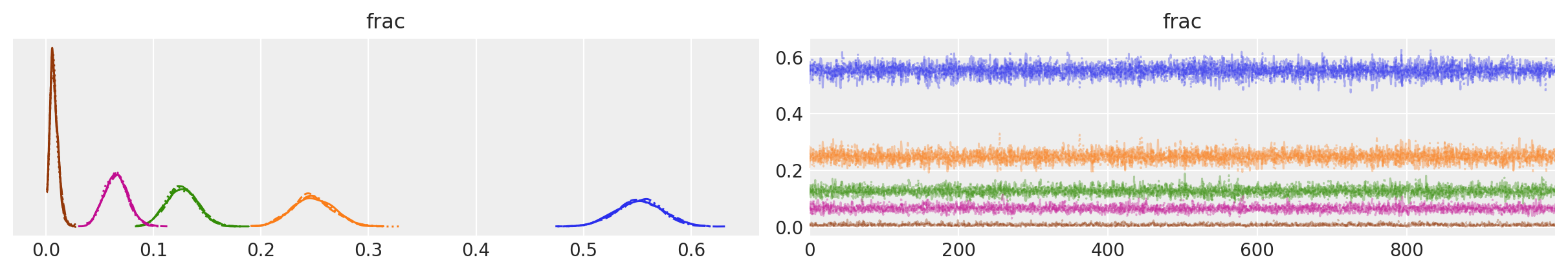
The trace plots look fairly good; visually, each parameter appears to be moving around the posterior well.

summary_multinomial = az.summary(trace_multinomial, var_names=["frac"])

summary_multinomial = summary_multinomial.assign(
    ess_bulk_per_sec=lambda x: x.ess_bulk / trace_multinomial.posterior.sampling_time,
)

summary_multinomial

	mean	sd	hdi_3%	hdi_97%	mcse_mean	mcse_sd	ess_bulk	ess_tail	r_hat	ess_bulk_per_sec
frac[pine]	0.552	0.022	0.510	0.591	0.0	0.0	5955.0	3480.0	1.0	2675.351076
frac[oak]	0.248	0.019	0.213	0.284	0.0	0.0	5428.0	3478.0	1.0	2438.590368
frac[ebony]	0.127	0.015	0.099	0.153	0.0	0.0	4773.0	3080.0	1.0	2144.324212
frac[rosewood]	0.065	0.011	0.045	0.086	0.0	0.0	3351.0	2680.0	1.0	1505.474636
frac[mahogany]	0.008	0.004	0.001	0.015	0.0	0.0	1341.0	1277.0	1.0	602.459411

Likewise, diagnostics in the parameter summary table all look fine. Here we’ve added a column estimating the effective sample size per second of sampling.

az.plot_forest(trace_multinomial, var_names=["frac"])
for j, (y_tick, frac_j) in enumerate(zip(plt.gca().get_yticks(), reversed(true_frac))):
    plt.vlines(frac_j, ymin=y_tick - 0.45, ymax=y_tick + 0.45, color="black", linestyle="--")

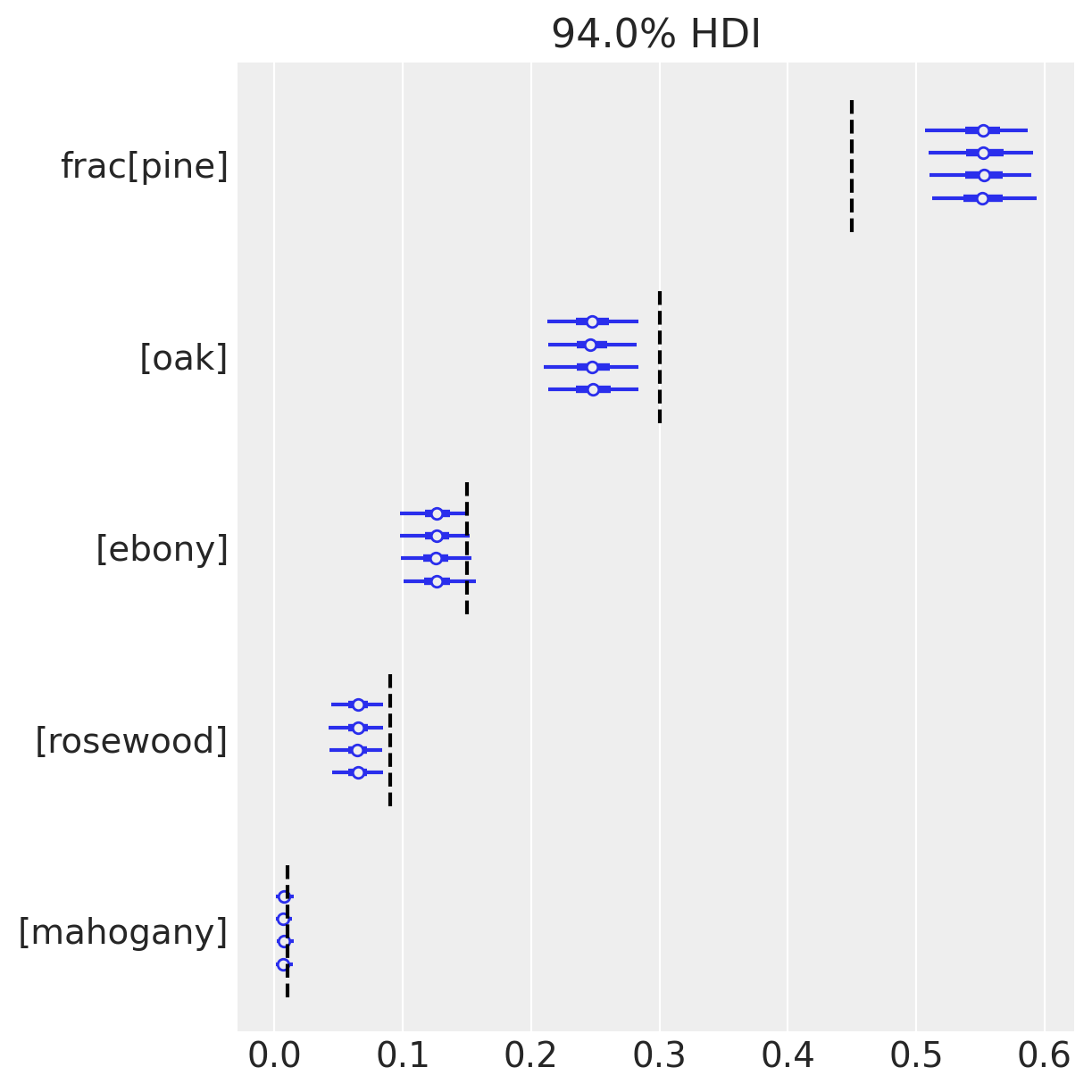
Here we’ve drawn a forest-plot, showing the mean and 94% HDIs from our posterior approximation. Interestingly, because we know what the underlying frequencies are for each species (dashed lines), we can comment on the accuracy of our inferences. And now the issues with our model become apparent; notice that the 94% HDIs don’t include the true values for tree species 0, 1, 3. We might have seen one HDI miss, but three???

…what’s going on?

Let’s troubleshoot this model using a posterior-predictive check, comparing our data to simulated data conditioned on our posterior estimates.

with model_multinomial:
    pp_samples = pm.sample_posterior_predictive(trace=trace_multinomial)

# Concatenate with InferenceData object
trace_multinomial.extend(pp_samples)

Sampling: [counts]

100.00% [4000/4000 00:00<00:00]

cmap = plt.get_cmap("tab10")

fig, axs = plt.subplots(k, 1, sharex=True, sharey=True, figsize=(6, 8))
for j, ax in enumerate(axs):
    c = cmap(j)
    ax.hist(
        trace_multinomial.posterior_predictive.counts.sel(tree=trees[j]).values.flatten(),
        bins=np.arange(total_count),
        histtype="step",
        color=c,
        density=True,
        label="Post.Pred.",
    )
    ax.hist(
        (trace_multinomial.observed_data.counts.sel(tree=trees[j]).values.flatten()),
        bins=np.arange(total_count),
        color=c,
        density=True,
        alpha=0.25,
        label="Observed",
    )
    ax.axvline(
        true_frac[j] * total_count,
        color=c,
        lw=1.0,
        alpha=0.45,
        label="True",
    )
    ax.annotate(
        f"{trees[j]}",
        xy=(0.96, 0.9),
        xycoords="axes fraction",
        ha="right",
        va="top",
        color=c,
    )

axs[-1].legend(loc="upper center", fontsize=10)
axs[-1].set_xlabel("Count")
axs[-1].set_yticks([0, 0.5, 1.0])
axs[-1].set_ylim(0, 0.6);

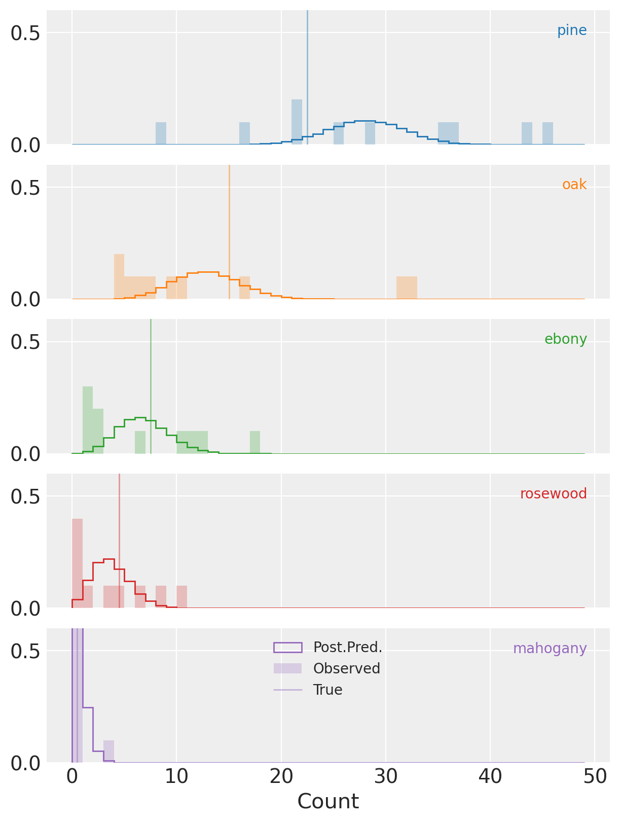
Here we’re plotting histograms of the predicted counts against the observed counts for each species.

(Notice that the y-axis isn’t full height and clips the distributions for species mahogany in purple.)

And now we can start to see why our posterior HDI deviates from the true parameters for three of five species (vertical lines). See that for all of the species the observed counts are frequently quite far from the predictions conditioned on the posterior distribution. This is particularly obvious for (e.g.) oak where we have one observation of more than 30 trees of this species, despite the posterior predicitive mass being concentrated far below that.

This is overdispersion at work, and a clear sign that we need to adjust our model to accommodate it.

Posterior predictive checks are one of the best ways to diagnose model misspecification, and this example is no different.

Dirichlet-Multinomial Model - Explicit Mixture

Let’s go ahead and model our data using the DM distribution.

For this model we’ll keep the same prior on the expected frequencies of each species, \(\mathrm{frac}\). We’ll also add a strictly positive parameter, \(\mathrm{conc}\), for the concentration.

In this iteration of our model we’ll explicitly include the latent multinomial probability, \(p_i\), modeling the \(\mathrm{true\_p}_i\) from our simulations (which we would not observe in the real world).

with pm.Model(coords=coords) as model_dm_explicit:
    frac = pm.Dirichlet("frac", a=np.ones(k), dims="tree")
    conc = pm.Lognormal("conc", mu=1, sigma=1)
    p = pm.Dirichlet("p", a=frac * conc, dims=("forest", "tree"))
    counts = pm.Multinomial(
        "counts", n=total_count, p=p, observed=observed_counts, dims=("forest", "tree")
    )

pm.model_to_graphviz(model_dm_explicit)

Compare this diagram to the first. Here the latent, Dirichlet distributed \(p\) separates the multinomial from the expected frequencies, \(\mathrm{frac}\), accounting for overdispersion of counts relative to the simple multinomial model.

with model_dm_explicit:
    trace_dm_explicit = pm.sample(chains=4, target_accept=0.9)

Auto-assigning NUTS sampler...
Initializing NUTS using jitter+adapt_diag...
Multiprocess sampling (4 chains in 4 jobs)
NUTS: [frac, conc, p]

100.00% [8000/8000 01:27<00:00 Sampling 4 chains, 16 divergences]

Sampling 4 chains for 1_000 tune and 1_000 draw iterations (4_000 + 4_000 draws total) took 87 seconds.
The rhat statistic is larger than 1.01 for some parameters. This indicates problems during sampling. See https://arxiv.org/abs/1903.08008 for details
The effective sample size per chain is smaller than 100 for some parameters.  A higher number is needed for reliable rhat and ess computation. See https://arxiv.org/abs/1903.08008 for details
There were 16 divergences after tuning. Increase `target_accept` or reparameterize.

Here we had to increase target_accept from 0.8 to 0.9 to not get drowned in divergences.

We also got a warning about the rhat statistic, although we’ll ignore it for now. More interesting is how much longer it took to sample this model than the first. This is partly because our model has an additional ~\((n \times k)\) parameters, but it seems like there are other geometric challenges for NUTS as well.

We’ll see if we can fix these in the next model, but for now let’s take a look at the traces.

az.plot_trace(data=trace_dm_explicit, var_names=["frac", "conc"]);

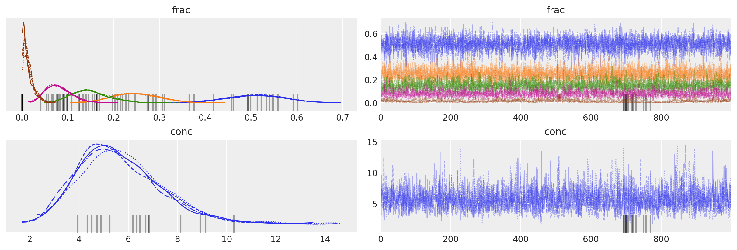
The divergences seem to occur when the estimated fraction of the rare species (mahogany) is very close to zero.

az.plot_forest(trace_dm_explicit, var_names=["frac"])
for j, (y_tick, frac_j) in enumerate(zip(plt.gca().get_yticks(), reversed(true_frac))):
    plt.vlines(frac_j, ymin=y_tick - 0.45, ymax=y_tick + 0.45, color="black", linestyle="--")

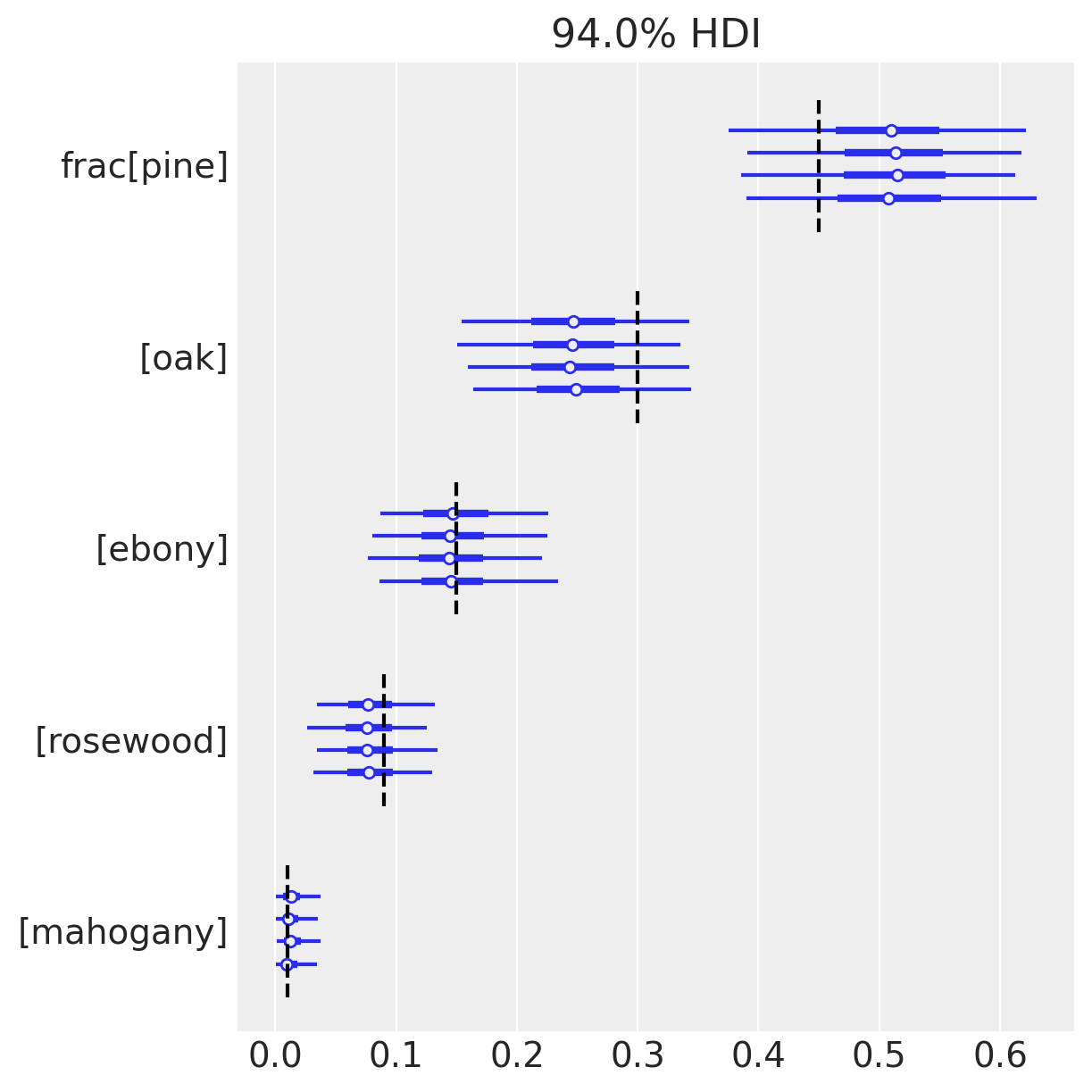
On the other hand, since we know the ground-truth for \(\mathrm{frac}\), we can congratulate ourselves that the HDIs include the true values for all of our species!

Modeling this mixture has made our inferences robust to the overdispersion of counts, while the plain multinomial is very sensitive. Notice that the HDI is much wider than before for each \(\mathrm{frac}_i\). In this case that makes the difference between correct and incorrect inferences.

summary_dm_explicit = az.summary(trace_dm_explicit, var_names=["frac", "conc"])
summary_dm_explicit = summary_dm_explicit.assign(
    ess_bulk_per_sec=lambda x: x.ess_bulk / trace_dm_explicit.posterior.sampling_time,
)

summary_dm_explicit

	mean	sd	hdi_3%	hdi_97%	mcse_mean	mcse_sd	ess_bulk	ess_tail	r_hat	ess_bulk_per_sec
frac[pine]	0.509	0.063	0.386	0.622	0.001	0.001	4102.0	3040.0	1.00	47.028042
frac[oak]	0.248	0.050	0.158	0.343	0.001	0.000	5036.0	2996.0	1.00	57.736036
frac[ebony]	0.149	0.040	0.082	0.227	0.001	0.000	3379.0	2915.0	1.00	38.739091
frac[rosewood]	0.080	0.028	0.031	0.131	0.001	0.000	2147.0	2488.0	1.00	24.614628
frac[mahogany]	0.014	0.012	0.000	0.036	0.001	0.001	69.0	109.0	1.04	0.791062
conc	5.712	1.741	2.729	8.872	0.036	0.026	2209.0	2082.0	1.00	25.325437

This is great, but we can do better. The slightly too large \(\hat{R}\) value for frac[mahogany] is a bit concerning, and it’s surprising that our \(\mathrm{ESS} \; \mathrm{sec}^{-1}\) is quite small.

Dirichlet-Multinomial Model - Marginalized

Happily, the Dirichlet distribution is conjugate to the multinomial and therefore there’s a convenient, closed-form for the marginalized distribution, i.e. the Dirichlet-multinomial distribution, which was added to PyMC in 3.11.0.

Let’s take advantage of this, marginalizing out the explicit latent parameter, \(p_i\), replacing the combination of this node and the multinomial with the DM to make an equivalent model.

with pm.Model(coords=coords) as model_dm_marginalized:
    frac = pm.Dirichlet("frac", a=np.ones(k), dims="tree")
    conc = pm.Lognormal("conc", mu=1, sigma=1)
    counts = pm.DirichletMultinomial(
        "counts", n=total_count, a=frac * conc, observed=observed_counts, dims=("forest", "tree")
    )

pm.model_to_graphviz(model_dm_marginalized)

The plate diagram shows that we’ve collapsed what had been the latent Dirichlet and the multinomial nodes together into a single DM node.

with model_dm_marginalized:
    trace_dm_marginalized = pm.sample(chains=4)

Auto-assigning NUTS sampler...
Initializing NUTS using jitter+adapt_diag...
Multiprocess sampling (4 chains in 4 jobs)
NUTS: [frac, conc]

100.00% [8000/8000 00:02<00:00 Sampling 4 chains, 0 divergences]

Sampling 4 chains for 1_000 tune and 1_000 draw iterations (4_000 + 4_000 draws total) took 2 seconds.

It samples much more quickly and without any of the warnings from before!

az.plot_trace(data=trace_dm_marginalized, var_names=["frac", "conc"]);

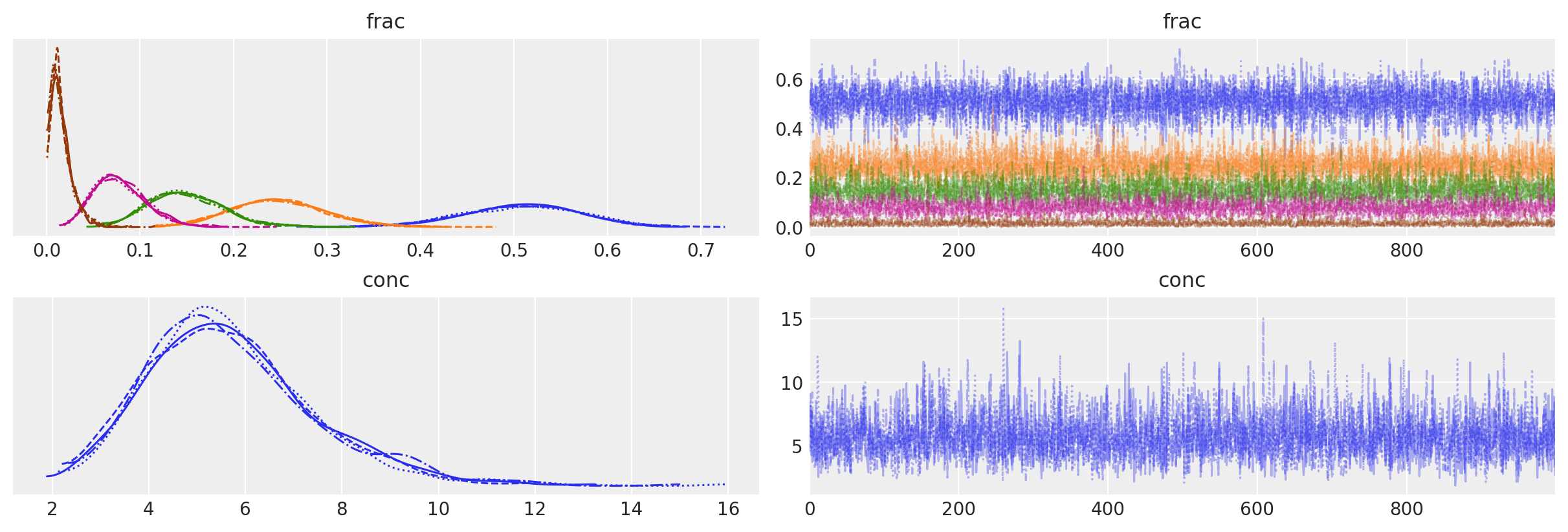
Trace plots look fuzzy and KDEs are clean.

summary_dm_marginalized = az.summary(trace_dm_marginalized, var_names=["frac", "conc"])
summary_dm_marginalized = summary_dm_marginalized.assign(
    ess_mean_per_sec=lambda x: x.ess_bulk / trace_dm_marginalized.posterior.sampling_time,
)
assert all(summary_dm_marginalized.r_hat < 1.03)

summary_dm_marginalized

	mean	sd	hdi_3%	hdi_97%	mcse_mean	mcse_sd	ess_bulk	ess_tail	r_hat	ess_mean_per_sec
frac[pine]	0.507	0.063	0.385	0.619	0.001	0.001	4330.0	2816.0	1.0	1870.135862
frac[oak]	0.248	0.051	0.150	0.341	0.001	0.000	6017.0	3571.0	1.0	2598.754615
frac[ebony]	0.150	0.040	0.080	0.226	0.001	0.000	4315.0	3296.0	1.0	1863.657331
frac[rosewood]	0.079	0.028	0.031	0.130	0.000	0.000	3027.0	2718.0	1.0	1307.367495
frac[mahogany]	0.016	0.011	0.001	0.036	0.000	0.000	2856.0	2172.0	1.0	1233.512245
conc	5.692	1.719	2.807	9.045	0.028	0.020	3594.0	2925.0	1.0	1552.255956

We see that \(\hat{R}\) is close to \(1\) everywhere and \(\mathrm{ESS} \; \mathrm{sec}^{-1}\) is much higher. Our reparameterization (marginalization) has greatly improved the sampling! (And, thankfully, the HDIs look similar to the other model.)

This all looks very good, but what if we didn’t have the ground-truth?

Posterior predictive checks to the rescue (again)!

with model_dm_marginalized:
    pp_samples = pm.sample_posterior_predictive(trace_dm_marginalized)

# Concatenate with InferenceData object
trace_dm_marginalized.extend(pp_samples)

Sampling: [counts]

5.53% [221/4000 00:00<00:00]

cmap = plt.get_cmap("tab10")

fig, axs = plt.subplots(k, 2, sharex=True, sharey=True, figsize=(8, 8))
for j, row in enumerate(axs):
    c = cmap(j)
    for _trace, ax in zip([trace_dm_marginalized, trace_multinomial], row):
        ax.hist(
            _trace.posterior_predictive.counts.sel(tree=trees[j]).values.flatten(),
            bins=np.arange(total_count),
            histtype="step",
            color=c,
            density=True,
            label="Post.Pred.",
        )
        ax.hist(
            (_trace.observed_data.counts.sel(tree=trees[j]).values.flatten()),
            bins=np.arange(total_count),
            color=c,
            density=True,
            alpha=0.25,
            label="Observed",
        )
        ax.axvline(
            true_frac[j] * total_count,
            color=c,
            lw=1.0,
            alpha=0.45,
            label="True",
        )
    row[1].annotate(
        f"{trees[j]}",
        xy=(0.96, 0.9),
        xycoords="axes fraction",
        ha="right",
        va="top",
        color=c,
    )

axs[-1, -1].legend(loc="upper center", fontsize=10)
axs[0, 1].set_title("Multinomial")
axs[0, 0].set_title("Dirichlet-multinomial")
axs[-1, 0].set_xlabel("Count")
axs[-1, 1].set_xlabel("Count")
axs[-1, 0].set_yticks([0, 0.5, 1.0])
axs[-1, 0].set_ylim(0, 0.6)
ax.set_ylim(0, 0.6);

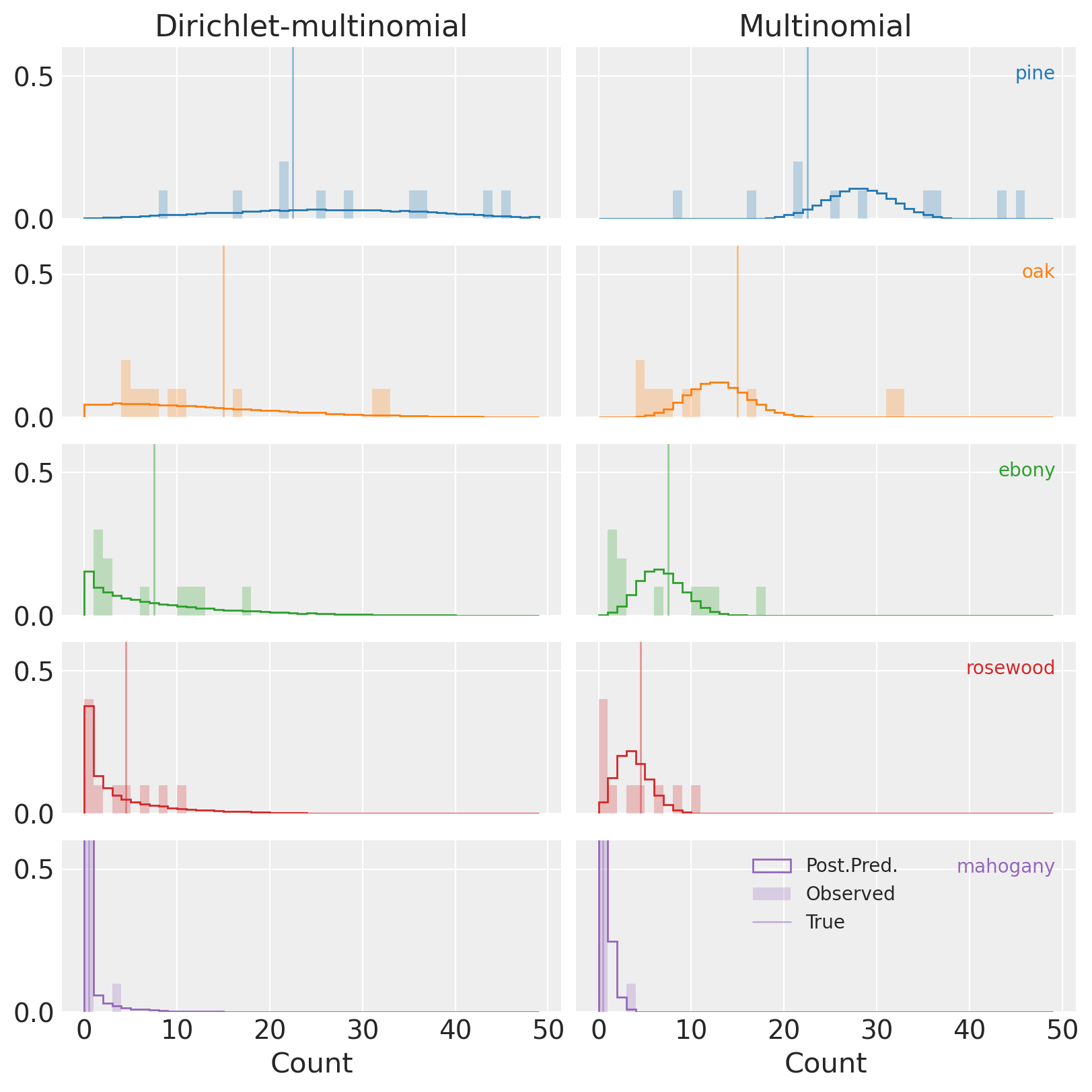
(Notice, again, that the y-axis isn’t full height, and clips the distributions for mahogany in purple.)

Compared to the multinomial (plots on the right), PPCs for the DM (left) show that the observed data is an entirely reasonable realization of our model. This is great news!

Model Comparison

Let’s go a step further and try to put a number on how much better our DM model is relative to the raw multinomial. We’ll use leave-one-out cross validation to compare the out-of-sample predictive ability of the two.

with model_multinomial:
    pm.compute_log_likelihood(trace_multinomial)

with model_dm_marginalized:
    pm.compute_log_likelihood(trace_dm_marginalized)

az.compare(
    {"multinomial": trace_multinomial, "dirichlet_multinomial": trace_dm_marginalized}, ic="loo"
)

100.00% [4000/4000 00:00<00:00]

100.00% [4000/4000 00:00<00:00]

/home/erik/mambaforge/envs/pymc_examples/lib/python3.11/site-packages/arviz/stats/stats.py:803: UserWarning: Estimated shape parameter of Pareto distribution is greater than 0.7 for one or more samples. You should consider using a more robust model, this is because importance sampling is less likely to work well if the marginal posterior and LOO posterior are very different. This is more likely to happen with a non-robust model and highly influential observations.
  warnings.warn(
/home/erik/mambaforge/envs/pymc_examples/lib/python3.11/site-packages/arviz/stats/stats.py:307: FutureWarning: Setting an item of incompatible dtype is deprecated and will raise in a future error of pandas. Value 'False' has dtype incompatible with float64, please explicitly cast to a compatible dtype first.
  df_comp.loc[val] = (
/home/erik/mambaforge/envs/pymc_examples/lib/python3.11/site-packages/arviz/stats/stats.py:307: FutureWarning: Setting an item of incompatible dtype is deprecated and will raise in a future error of pandas. Value 'log' has dtype incompatible with float64, please explicitly cast to a compatible dtype first.
  df_comp.loc[val] = (

	rank	elpd_loo	p_loo	elpd_diff	weight	se	dse	warning	scale
dirichlet_multinomial	0	-96.773440	4.126392	0.000000	1.000000e+00	6.823526	0.000000	False	log
multinomial	1	-174.447424	24.065196	77.673984	2.735590e-13	24.884526	23.983963	True	log

Unsurprisingly, the DM outclasses the multinomial by a mile, assigning a weight of 100% to the over-dispersed model. While the warning=True flag for the multinomial distribution indicates that the numerical value cannot be fully trusted, the large difference in elpd_loo is further confirmation that between the two, the DM should be greatly favored for prediction, parameter inference, etc.

Conclusions

Obviously the DM is not a perfect model in every case, but it is often a better choice than the multinomial, much more robust while taking on just one additional parameter.

There are a number of shortcomings to the DM that we should keep in mind when selecting a model. The biggest problem is that, while more flexible than the multinomial, the DM still ignores the possibility of underlying correlations between categories. If one of our tree species relies on another, for instance, the model we’ve used here will not effectively account for this. In that case, swapping the vanilla Dirichlet distribution for something fancier (e.g. the Generalized Dirichlet or Logistic-Multivariate Normal) may be worth considering.

References

Authors

• Authored by Byron J. Smith on Jan, 2021 (pymc-examples#18)

• Updated by Abhipsha Das and Oriol Abril-Pla on August, 2021 (pymc-examples#212)

• Updated to PyMC v5 by Erik Werner on Oct, 2023 (pymc-examples#581)

Watermark

%load_ext watermark
%watermark -n -u -v -iv -w -p pytensor,xarray

Last updated: Thu Oct 05 2023

Python implementation: CPython
Python version       : 3.11.6
IPython version      : 8.16.1

pytensor: 2.17.1
xarray  : 2023.9.0

numpy     : 1.25.2
arviz     : 0.16.1
scipy     : 1.11.3
pymc      : 5.9.0
matplotlib: 3.8.0

Watermark: 2.4.3