Automatic marginalization of discrete variables#
PyMC is very amendable to sampling models with discrete latent variables. But if you insist on using the NUTS sampler exclusively, you will need to get rid of your discrete variables somehow. The best way to do this is by marginalizing them out, as then you benefit from Rao-Blackwell’s theorem and get a lower variance estimate of your parameters.
Formally the argument goes like this, samplers can be understood as approximating the expectation \(\mathbb{E}_{p(x, z)}[f(x, z)]\) for some function \(f\) with respect to a distribution \(p(x, z)\). By law of total expectation we know that
Letting \(g(z) = \mathbb{E}_{p(x \mid z)}\left[f(x, z)\right]\), we know by law of total variance that
Because the expectation is over a variance it must always be positive, and thus we know
Intuitively, marginalizing variables in your model lets you use \(g\) instead of \(f\). This lower variance manifests most directly in lower Monte-Carlo standard error (mcse), and indirectly in a generally higher effective sample size (ESS).
Unfortunately, the computation to do this is often tedious and unintuitive. Luckily, pymc-experimental now supports a way to do this work automatically!
import arviz as az
import matplotlib.pyplot as plt
import numpy as np
import pandas as pd
import pymc as pm
import pytensor.tensor as pt
Attention
This notebook uses libraries that are not PyMC dependencies and therefore need to be installed specifically to run this notebook. Open the dropdown below for extra guidance.
Extra dependencies install instructions
In order to run this notebook (either locally or on binder) you won’t only need a working PyMC installation with all optional dependencies, but also to install some extra dependencies. For advise on installing PyMC itself, please refer to Installation
You can install these dependencies with your preferred package manager, we provide as an example the pip and conda commands below.
$ pip install pymc-experimental
Note that if you want (or need) to install the packages from inside the notebook instead of the command line, you can install the packages by running a variation of the pip command:
import sys
!{sys.executable} -m pip install pymc-experimental
You should not run !pip install as it might install the package in a different
environment and not be available from the Jupyter notebook even if installed.
Another alternative is using conda instead:
$ conda install pymc-experimental
when installing scientific python packages with conda, we recommend using conda forge
import pymc_experimental as pmx
%config InlineBackend.figure_format = 'retina'  # high resolution figures
az.style.use("arviz-darkgrid")
rng = np.random.default_rng(32)
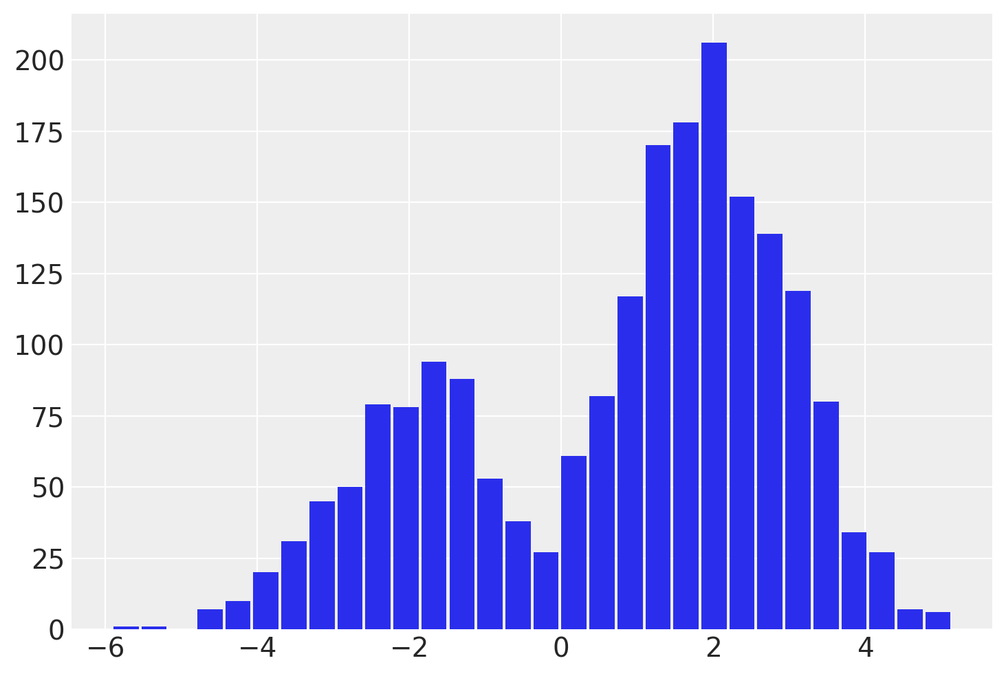
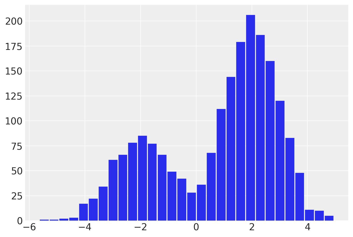
As a motivating example, consider a gaussian mixture model
Gaussian Mixture model#
There are two ways to specify the same model. One where the choice of mixture is explicit.
mu = pt.as_tensor([-2.0, 2.0])

with pmx.MarginalModel() as explicit_mixture:
    idx = pm.Bernoulli("idx", 0.7)
    y = pm.Normal("y", mu=mu[idx], sigma=1.0)
The other way is where we use the built-in NormalMixture distribution. Here the mixture assignment is not an explicit variable in our model. There is nothing unique about the first model other than we initialize it with pmx.MarginalModel instead of pm.Model. This different class is what will allow us to marginalize out variables later.
with pm.Model() as prebuilt_mixture:
    y = pm.NormalMixture("y", w=[0.3, 0.7], mu=[-2, 2])
with prebuilt_mixture:
    idata = pm.sample(draws=2000, chains=4, random_seed=rng)

az.summary(idata)
Auto-assigning NUTS sampler...
Initializing NUTS using jitter+adapt_diag...
Multiprocess sampling (4 chains in 2 jobs)
NUTS: [y]
Sampling 4 chains for 1_000 tune and 2_000 draw iterations (4_000 + 8_000 draws total) took 10 seconds.
The rhat statistic is larger than 1.01 for some parameters. This indicates problems during sampling. See https://arxiv.org/abs/1903.08008 for details
| mean | sd | hdi_3% | hdi_97% | mcse_mean | mcse_sd | ess_bulk | ess_tail | r_hat | |
|---|---|---|---|---|---|---|---|---|---|
| y | 0.863 | 2.08 | -3.138 | 3.832 | 0.095 | 0.067 | 555.0 | 1829.0 | 1.01 |
with explicit_mixture:
    idata = pm.sample(draws=2000, chains=4, random_seed=rng)

az.summary(idata)
Multiprocess sampling (4 chains in 2 jobs)
CompoundStep
>BinaryGibbsMetropolis: [idx]
>NUTS: [y]
Sampling 4 chains for 1_000 tune and 2_000 draw iterations (4_000 + 8_000 draws total) took 10 seconds.
The rhat statistic is larger than 1.01 for some parameters. This indicates problems during sampling. See https://arxiv.org/abs/1903.08008 for details
The effective sample size per chain is smaller than 100 for some parameters.  A higher number is needed for reliable rhat and ess computation. See https://arxiv.org/abs/1903.08008 for details
| mean | sd | hdi_3% | hdi_97% | mcse_mean | mcse_sd | ess_bulk | ess_tail | r_hat | |
|---|---|---|---|---|---|---|---|---|---|
| idx | 0.718 | 0.450 | 0.000 | 1.000 | 0.028 | 0.020 | 252.0 | 252.0 | 1.02 |
| y | 0.875 | 2.068 | -3.191 | 3.766 | 0.122 | 0.087 | 379.0 | 1397.0 | 1.01 |
We can immediately see that the marginalized model has a higher ESS. Let’s now marginalize out the choice and see what it changes in our model.
explicit_mixture.marginalize(["idx"])
with explicit_mixture:
    idata = pm.sample(draws=2000, chains=4, random_seed=rng)

az.summary(idata)
Auto-assigning NUTS sampler...
Initializing NUTS using jitter+adapt_diag...
Multiprocess sampling (4 chains in 2 jobs)
NUTS: [y]
Sampling 4 chains for 1_000 tune and 2_000 draw iterations (4_000 + 8_000 draws total) took 10 seconds.
| mean | sd | hdi_3% | hdi_97% | mcse_mean | mcse_sd | ess_bulk | ess_tail | r_hat | |
|---|---|---|---|---|---|---|---|---|---|
| y | 0.731 | 2.102 | -3.202 | 3.811 | 0.099 | 0.07 | 567.0 | 2251.0 | 1.01 |
As we can see, the idx variable is gone now. We also were able to use the NUTS sampler, and the ESS has improved.
But MarginalModel has a distinct advantage. It still knows about the discrete variables that were marginalized out, and we can obtain estimates for the posterior of idx given the other variables. We do this using the recover_marginals method.
explicit_mixture.recover_marginals(idata, random_seed=rng);
az.summary(idata)
| mean | sd | hdi_3% | hdi_97% | mcse_mean | mcse_sd | ess_bulk | ess_tail | r_hat | |
|---|---|---|---|---|---|---|---|---|---|
| y | 0.731 | 2.102 | -3.202 | 3.811 | 0.099 | 0.070 | 567.0 | 2251.0 | 1.01 |
| idx | 0.683 | 0.465 | 0.000 | 1.000 | 0.023 | 0.016 | 420.0 | 420.0 | 1.01 |
| lp_idx[0] | -6.064 | 5.242 | -14.296 | -0.000 | 0.227 | 0.160 | 567.0 | 2251.0 | 1.01 |
| lp_idx[1] | -2.294 | 3.931 | -10.548 | -0.000 | 0.173 | 0.122 | 567.0 | 2251.0 | 1.01 |
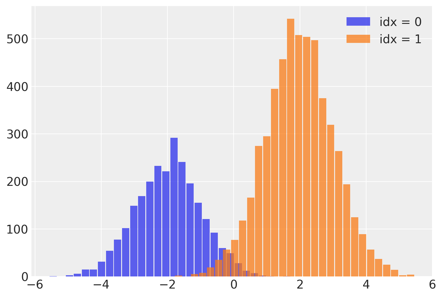
This idx variable lets us recover the mixture assignment variable after running the NUTS sampler! We can split out the samples of y by reading off the mixture label from the associated idx for each sample.
# fmt: off
post = idata.posterior
plt.hist(
    post.where(post.idx == 0).y.values.reshape(-1),
    bins=30,
    rwidth=0.9,
    alpha=0.75,
    label='idx = 0',
)
plt.hist(
    post.where(post.idx == 1).y.values.reshape(-1),
    bins=30,
    rwidth=0.9,
    alpha=0.75,
    label='idx = 1'
)
# fmt: on
plt.legend();
One important thing to notice is that this discrete variable has a lower ESS, and particularly so for the tail. This means idx might not be estimated well particularly for the tails. If this is important, I recommend using the lp_idx instead, which is the log-probability of idx given sample values on each iteration. The benefits of working with lp_idx will explored further in the next example.
Coal mining model#
The same methods work for the Coal mining switchpoint model as well. The coal mining dataset records the number of coal mining disasters in the UK between 1851 and 1962. The time series dataset captures a time when mining safety regulations are being introduced, we try to estimate when this occurred using a discrete switchpoint variable.
# fmt: off
disaster_data = pd.Series(
    [4, 5, 4, 0, 1, 4, 3, 4, 0, 6, 3, 3, 4, 0, 2, 6,
    3, 3, 5, 4, 5, 3, 1, 4, 4, 1, 5, 5, 3, 4, 2, 5,
    2, 2, 3, 4, 2, 1, 3, np.nan, 2, 1, 1, 1, 1, 3, 0, 0,
    1, 0, 1, 1, 0, 0, 3, 1, 0, 3, 2, 2, 0, 1, 1, 1,
    0, 1, 0, 1, 0, 0, 0, 2, 1, 0, 0, 0, 1, 1, 0, 2,
    3, 3, 1, np.nan, 2, 1, 1, 1, 1, 2, 4, 2, 0, 0, 1, 4,
    0, 0, 0, 1, 0, 0, 0, 0, 0, 1, 0, 0, 1, 0, 1]
)

# fmt: on
years = np.arange(1851, 1962)

with pmx.MarginalModel() as disaster_model:
    switchpoint = pm.DiscreteUniform("switchpoint", lower=years.min(), upper=years.max())
    early_rate = pm.Exponential("early_rate", 1.0, initval=3)
    late_rate = pm.Exponential("late_rate", 1.0, initval=1)
    rate = pm.math.switch(switchpoint >= years, early_rate, late_rate)
    disasters = pm.Poisson("disasters", rate, observed=disaster_data)
/home/zv/upstream/pymc/pymc/model/core.py:1307: RuntimeWarning: invalid value encountered in cast
  data = convert_observed_data(data).astype(rv_var.dtype)
/home/zv/upstream/pymc/pymc/model/core.py:1321: ImputationWarning: Data in disasters contains missing values and will be automatically imputed from the sampling distribution.
  warnings.warn(impute_message, ImputationWarning)
We will sample the model both before and after we marginalize out the switchpoint variable
Multiprocess sampling (2 chains in 2 jobs)
CompoundStep
>CompoundStep
>>Metropolis: [switchpoint]
>>Metropolis: [disasters_unobserved]
>NUTS: [early_rate, late_rate]
Sampling 2 chains for 1_000 tune and 1_000 draw iterations (2_000 + 2_000 draws total) took 8 seconds.
We recommend running at least 4 chains for robust computation of convergence diagnostics
/home/zv/upstream/pymc-experimental/pymc_experimental/model/marginal_model.py:169: UserWarning: There are multiple dependent variables in a FiniteDiscreteMarginalRV. Their joint logp terms will be assigned to the first RV: disasters_unobserved
  warnings.warn(
Multiprocess sampling (2 chains in 2 jobs)
CompoundStep
>NUTS: [early_rate, late_rate]
>Metropolis: [disasters_unobserved]
Sampling 2 chains for 1_000 tune and 1_000 draw iterations (2_000 + 2_000 draws total) took 191 seconds.
We recommend running at least 4 chains for robust computation of convergence diagnostics
az.summary(before_marg, var_names=["~disasters"], filter_vars="like")
| mean | sd | hdi_3% | hdi_97% | mcse_mean | mcse_sd | ess_bulk | ess_tail | r_hat | |
|---|---|---|---|---|---|---|---|---|---|
| switchpoint | 1890.224 | 2.657 | 1886.000 | 1896.000 | 0.192 | 0.136 | 201.0 | 171.0 | 1.0 |
| early_rate | 3.085 | 0.279 | 2.598 | 3.636 | 0.007 | 0.005 | 1493.0 | 1255.0 | 1.0 |
| late_rate | 0.927 | 0.114 | 0.715 | 1.143 | 0.003 | 0.002 | 1136.0 | 1317.0 | 1.0 |
az.summary(after_marg, var_names=["~disasters"], filter_vars="like")
| mean | sd | hdi_3% | hdi_97% | mcse_mean | mcse_sd | ess_bulk | ess_tail | r_hat | |
|---|---|---|---|---|---|---|---|---|---|
| early_rate | 3.077 | 0.289 | 2.529 | 3.606 | 0.007 | 0.005 | 1734.0 | 1150.0 | 1.0 |
| late_rate | 0.932 | 0.113 | 0.725 | 1.150 | 0.003 | 0.002 | 1871.0 | 1403.0 | 1.0 |
As before, the ESS improved massively
Finally, let us recover the switchpoint variable
disaster_model.recover_marginals(after_marg);
az.summary(after_marg, var_names=["~disasters", "~lp"], filter_vars="like")
| mean | sd | hdi_3% | hdi_97% | mcse_mean | mcse_sd | ess_bulk | ess_tail | r_hat | |
|---|---|---|---|---|---|---|---|---|---|
| early_rate | 3.077 | 0.289 | 2.529 | 3.606 | 0.007 | 0.005 | 1734.0 | 1150.0 | 1.00 |
| late_rate | 0.932 | 0.113 | 0.725 | 1.150 | 0.003 | 0.002 | 1871.0 | 1403.0 | 1.00 |
| switchpoint | 1889.764 | 2.458 | 1886.000 | 1894.000 | 0.070 | 0.050 | 1190.0 | 1883.0 | 1.01 |
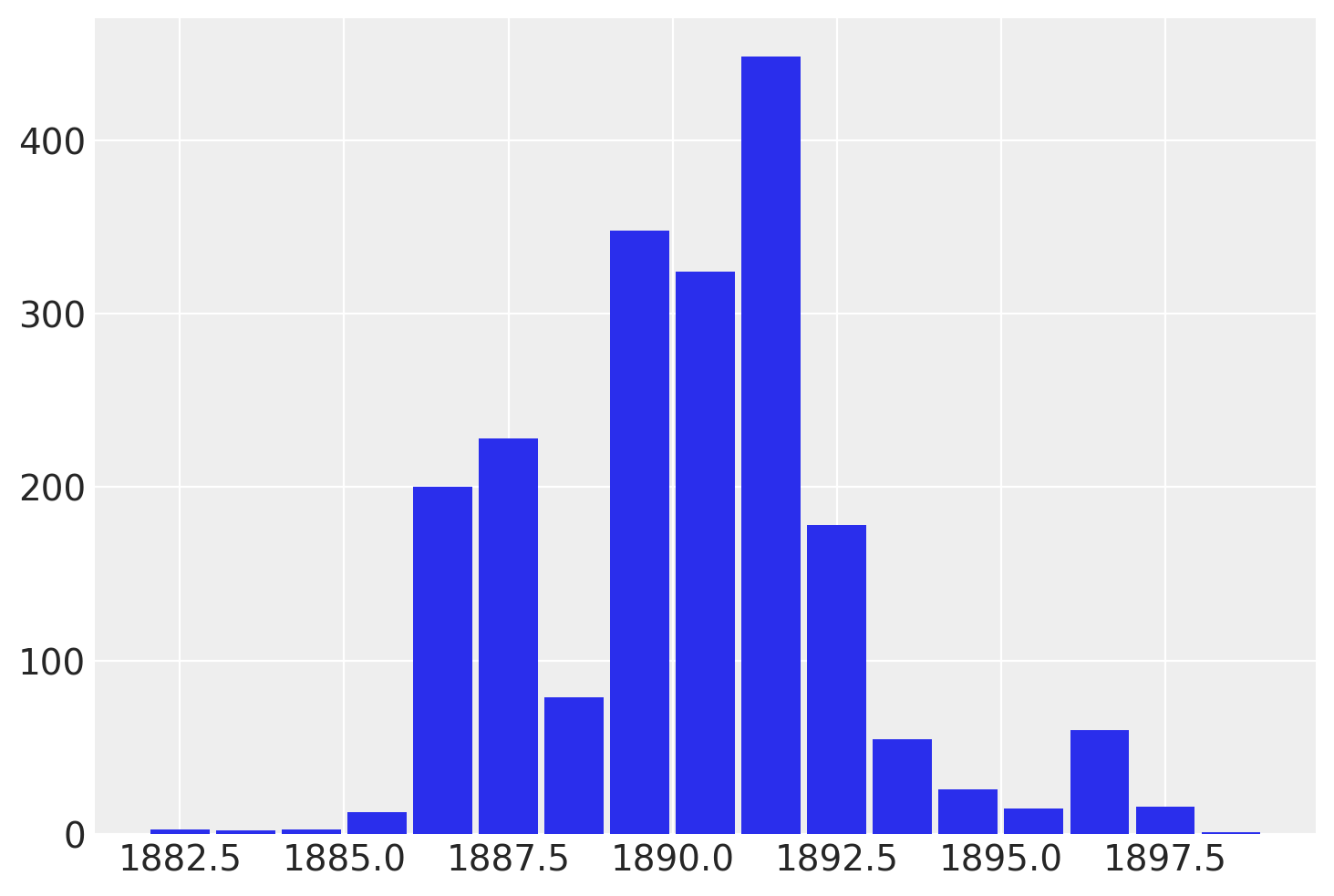
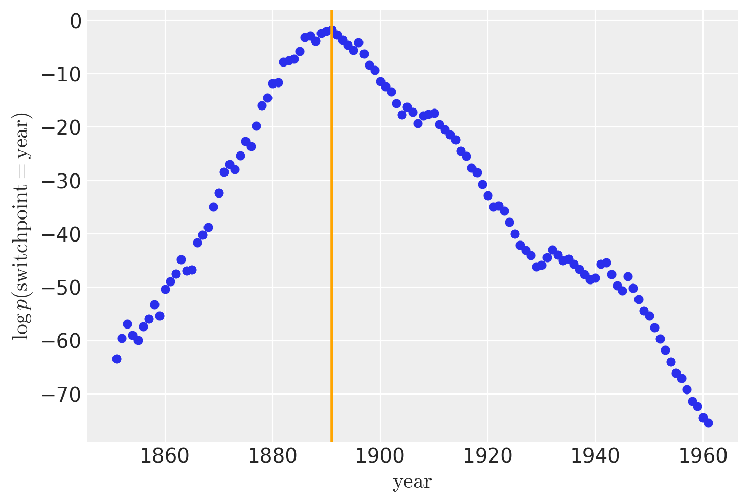
While recover_marginals is able to sample the discrete variables that were marginalized out. The probabilities associated with each draw often offer a cleaner estimate of the discrete variable. Particularly for lower probability values. This is best illustrated by comparing the histogram of the sampled values with the plot of the log-probabilities.
lp_switchpoint = after_marg.posterior.lp_switchpoint.mean(dim=["chain", "draw"])
x_max = years[lp_switchpoint.argmax()]

plt.scatter(years, lp_switchpoint)
plt.axvline(x=x_max, c="orange")
plt.xlabel(r"$\mathrm{year}$")
plt.ylabel(r"$\log p(\mathrm{switchpoint}=\mathrm{year})$");
By plotting a histogram of sampled values instead of working with the log-probabilities directly, we are left with noisier and more incomplete exploration of the underlying discrete distribution.
References#
Watermark#
%load_ext watermark
%watermark -n -u -v -iv -w -p pytensor,xarray
Last updated: Sat Feb 10 2024

Python implementation: CPython
Python version       : 3.11.6
IPython version      : 8.20.0

pytensor: 2.18.6
xarray  : 2023.11.0

pymc             : 5.11
numpy            : 1.26.3
pytensor         : 2.18.6
pymc_experimental: 0.0.15
arviz            : 0.17.0
pandas           : 2.1.4
matplotlib       : 3.8.2

Watermark: 2.4.3
License notice#
All the notebooks in this example gallery are provided under the MIT License which allows modification, and redistribution for any use provided the copyright and license notices are preserved.
Citing PyMC examples#
To cite this notebook, use the DOI provided by Zenodo for the pymc-examples repository.
Important
Many notebooks are adapted from other sources: blogs, books… In such cases you should cite the original source as well.
Also remember to cite the relevant libraries used by your code.
Here is an citation template in bibtex:
@incollection{citekey,
  author    = "<notebook authors, see above>",
  title     = "<notebook title>",
  editor    = "PyMC Team",
  booktitle = "PyMC examples",
  doi       = "10.5281/zenodo.5654871"
}
which once rendered could look like:
