


Heteroscedastic Bayesian Robust Regression#
import os
import warnings

import arviz as az
import matplotlib.pyplot as plt
import numpy as np
import pandas as pd
import pymc as pm
RANDOM_SEED = 8927
rng = np.random.default_rng(RANDOM_SEED)
az.style.use("arviz-variat")
# suppress pip-installed PyTensor BLAS warning (not actionable without conda)
warnings.filterwarnings("ignore", message="PyTensor could not link to a BLAS")
Motivation#
The PyMC gallery has two robust regression notebooks: one with a Student-t likelihood (pymc-examples:GLM-robust) and one with the Hogg (2010) signal-vs-noise mixture (pymc-examples:GLM-robust-with-outlier-detection). Both protect against vertical outliers (points with unusual response values), but neither defends against leverage points: observations far from the bulk of the predictor space, which can drag the regression line even under a heavy-tailed likelihood.
[Peña et al., 2009] show that this is not specific to the Student-t:
Theorem 1. No i.i.d. error model (Normal, Student-t, Laplace, or any scale mixture of normals) can achieve formal Kullback-Leibler robustness. A single observation moved far enough in the predictor space distorts the posterior of \(\beta\) without bound.
Theorem 2. A heteroscedastic model in which each observation receives a data-driven weight \(w_i \in (0, 1]\) does achieve KL-robustness.
We implement that model here and compare it against the Normal and Student-t baselines on three classic datasets.
Model#
Following the initials of the authors, we refer to the Peña-Zamar-Yan model as PZY in the rest of the notebook. The PZY likelihood modifies Laplace regression by scaling the noise parameter observation-by-observation:
Observations near the bulk of the data get \(w_i = 1\) and are fit normally. Observations far from the bulk get \(w_i < 1\), which inflates their noise scale and downweights their influence on the posterior of \(\beta\). For example, a point with \(w_i = 0.1\) has its scale multiplied by 10; its likelihood is therefore much wider and pulls the regression line much less than a clean point would.
Peña et al. [2009] use the improper noninformative prior \(\pi(\beta, \sigma^2) \propto 1/\sigma^2\) in all their examples. We use the closest PyMC equivalents: \(\alpha, \beta_j \sim \text{Flat}\) and \(\sigma \sim \text{HalfFlat}\). The likelihood is informative enough that the posterior is proper and NUTS samples it cleanly. For the Student-t baseline we add \(\nu \sim \text{Exponential}(1/30)\), the same prior used in pymc-examples:GLM-robust.
Computing the weights#
Given the augmented matrix \(Z = [y, X]\) (no intercept column):
Robust location: \(m_j = \text{median}(z_{ij})\) for each coordinate \(j\).
Robust scale: \(s_j = \text{median}(|z_{ij} - m_j|)\), floored at \(\varepsilon\).
Quadrant correlation matrix \(R\): following Huber [1981], entry \((j,k)\) is the Pearson correlation between the sign vectors \(\text{sign}(z_{j} - m_j)\) and \(\text{sign}(z_{k} - m_k)\).
Robust covariance proxy: \(C = D R D\) where \(D = \text{diag}(s_1,\ldots,s_{p+1})\).
Robust Mahalanobis distance: \(d_i = \sqrt{(z_i - m)^\top C^{-1}(z_i - m)}\).
Cutoff: \(a = \text{median}(d) + k \cdot \text{MAD}(d)\), tuning parameter \(k > 0\).
Weights:
The weights are computed once before MCMC. They are deterministic functions
of the data, not sampled random variables. The PyMC model wraps them in
Data so they appear in the graph alongside the design matrix.
def _quadrant_correlation(Z, medians):
    """Quadrant-correlation matrix as defined in {cite:p}`huber1981robust` and
    used by Peña-Zamar-Yan: the Pearson correlation between the sign vectors
    sign(z_j - m_j) and sign(z_k - m_k)."""
    signs = np.sign(Z - medians)
    centered = signs - signs.mean(axis=0)
    std = centered.std(axis=0, ddof=0)
    std[std == 0] = 1.0
    normed = centered / std
    R = (normed.T @ normed) / signs.shape[0]
    np.fill_diagonal(R, 1.0)
    return R


def pzy_weights(X, y, k=2.0, eps=1e-8):
    """Peña-Zamar-Yan (2009) heteroscedastic weights.

    Parameters
    ----------
    X : ndarray (n, p)  design matrix without intercept
    y : ndarray (n,)
    k : float           cutoff multiplier on MAD of distances
    eps : float         floor on coordinate MAD values

    Returns
    -------
    weights : ndarray (n,) in (0, 1]
    info    : dict with keys 'distances', 'cutoff', 'location'
    """
    Z = np.column_stack([y, X])
    location = np.median(Z, axis=0)
    scale = np.maximum(np.median(np.abs(Z - location), axis=0), eps)
    R = _quadrant_correlation(Z, location)
    C = np.diag(scale) @ R @ np.diag(scale)
    diff = Z - location
    d_sq = np.einsum("ij,jk,ik->i", diff, np.linalg.pinv(C), diff)
    distances = np.sqrt(np.maximum(d_sq, 0.0))
    med_d = np.median(distances)
    cutoff = med_d + k * np.median(np.abs(distances - med_d))
    above = distances > cutoff
    weights = np.ones(len(y))
    weights[above] = 1.0 / np.sqrt(1.0 + distances[above] ** 2 - cutoff**2)
    return weights, {"distances": distances, "cutoff": cutoff, "location": location}
def _fit(model, draws=2000, tune=2000, target_accept=0.9, max_treedepth=10):
    """Sample with NUTS, instantiating the step method explicitly so that
    target_accept and max_treedepth are reliably honored."""
    with model:
        step = pm.NUTS(target_accept=target_accept, max_treedepth=max_treedepth)
        return pm.sample(draws=draws, tune=tune, step=step, random_seed=RANDOM_SEED)


def fit_normal(X, y, predictor_names, **kw):
    n, _ = X.shape
    coords = {"predictor": predictor_names, "obs": np.arange(n)}
    with pm.Model(coords=coords) as model:
        intercept = pm.Flat("intercept")
        beta = pm.Flat("beta", dims="predictor")
        sigma = pm.HalfFlat("sigma")
        mu = intercept + pm.math.dot(pm.Data("X", X, dims=("obs", "predictor")), beta)
        pm.Normal("y_obs", mu=mu, sigma=sigma, observed=y, dims="obs")
    return _fit(model, **kw), model


def fit_studentt(X, y, predictor_names, **kw):
    n, _ = X.shape
    coords = {"predictor": predictor_names, "obs": np.arange(n)}
    with pm.Model(coords=coords) as model:
        intercept = pm.Flat("intercept")
        beta = pm.Flat("beta", dims="predictor")
        sigma = pm.HalfFlat("sigma")
        nu = pm.Exponential("nu", lam=1.0 / 30.0)
        mu = intercept + pm.math.dot(pm.Data("X", X, dims=("obs", "predictor")), beta)
        pm.StudentT("y_obs", nu=nu, mu=mu, sigma=sigma, observed=y, dims="obs")
    # The Exponential(1/30) prior on nu produces a heavy-tailed posterior with
    # difficult geometry; bump target_accept and max_treedepth to keep chains stable.
    kw.setdefault("target_accept", 0.95)
    kw.setdefault("max_treedepth", 15)
    return _fit(model, **kw), model


def fit_pzy(X, y, predictor_names, k=2.0, **kw):
    weights, info = pzy_weights(X, y, k=k)
    n, _ = X.shape
    coords = {"predictor": predictor_names, "obs": np.arange(n)}
    with pm.Model(coords=coords) as model:
        intercept = pm.Flat("intercept")
        beta = pm.Flat("beta", dims="predictor")
        sigma = pm.HalfFlat("sigma")
        w = pm.Data("weights", weights, dims="obs")
        mu = intercept + pm.math.dot(pm.Data("X", X, dims=("obs", "predictor")), beta)
        pm.Laplace("y_obs", mu=mu, b=sigma / w, observed=y, dims="obs")
    # Heavily downweighted points (small w) inflate b = sigma/w and create
    # funnel-like geometry; deeper trees help NUTS traverse it without warnings.
    kw.setdefault("target_accept", 0.95)
    kw.setdefault("max_treedepth", 15)
    return _fit(model, **kw), model, weights, info


def _slope_hdi(idata, pred, hdi_prob=0.95):
    """Posterior mean and HDI for a named coefficient. Flattens chains for the mean.
    The default 95% level matches the credible intervals reported in
    {cite:p}`pena2009bayesian`."""
    post = idata.posterior["beta"].sel(predictor=pred).values.ravel()
    hdi = az.hdi(idata, var_names=["beta"], prob=hdi_prob)["beta"].sel(predictor=pred)
    return post.mean(), float(hdi.isel(ci_bound=0)), float(hdi.isel(ci_bound=1))


def _plot_dataset(
    X_col,
    y,
    idata_dict,
    pred,
    weights,
    df_labels=None,
    xlabel="x",
    ylabel="response",
    title="",
    n_lines=200,
):
    fig, axes = plt.subplots(1, 2, figsize=(12, 5))
    colors = {"Normal": "C0", "Student-t": "C1", "PZY": "C2"}

    # scatter + posterior regression lines
    ax = axes[0]
    x_line = np.linspace(X_col.min(), X_col.max(), 200).reshape(-1, 1)
    for name, idata in idata_dict.items():
        a_post = idata.posterior["intercept"].values.ravel()
        b_post = idata.posterior["beta"].sel(predictor=pred).values.ravel()
        n_draw = min(n_lines, len(a_post))
        idx = rng.choice(len(a_post), n_draw, replace=False)
        for i in idx:
            ax.plot(x_line, a_post[i] + b_post[i] * x_line, color=colors[name], alpha=0.03, lw=0.8)
        ax.plot(
            x_line, a_post.mean() + b_post.mean() * x_line, color=colors[name], lw=2, label=name
        )
    low_w = weights < 1.0
    ax.scatter(X_col, y, color="gray", s=25, zorder=3)
    ax.scatter(
        X_col[low_w], y[low_w], color="C1", s=55, zorder=4, marker="^", label="leverage (w < 1)"
    )
    if df_labels is not None:
        for i in np.where(low_w)[0]:
            ax.annotate(
                df_labels.iloc[i],
                (X_col[i], y[i]),
                fontsize=7,
                xytext=(4, 0),
                textcoords="offset points",
            )
    ax.set_xlabel(xlabel)
    ax.set_ylabel(ylabel)
    ax.set_title(title)
    ax.legend(fontsize=8)

    # HDI comparison
    ax = axes[1]
    for i, (name, idata) in enumerate(idata_dict.items()):
        mean, lo, hi = _slope_hdi(idata, pred)
        ax.errorbar(
            mean, i, xerr=[[mean - lo], [hi - mean]], fmt="o", color=colors[name], capsize=5
        )
    ax.set_yticks(range(len(idata_dict)))
    ax.set_yticklabels(list(idata_dict.keys()))
    ax.set_xlabel("slope  (95 % CI)")
    ax.set_title(f"Slope posterior: {title}")
    ax.axvline(0, color="gray", ls="--", lw=0.8)
Toy demonstration#
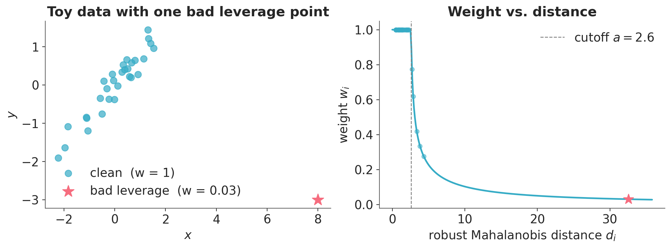
We start with a synthetic example. Draw 30 clean points from the line \(y = 0.8\,x\) plus small noise, then add one bad leverage point: far from the bulk in \(x\)-space, and far from the true line. Points within the cutoff distance \(a\) get weight 1; points beyond it get a smaller weight that decreases as \(d_i\) grows.
n_clean = 30
X_toy = rng.normal(0, 1, (n_clean, 1))
y_toy = 0.8 * X_toy[:, 0] + rng.normal(0, 0.3, n_clean)
# bad leverage point: large x, response inconsistent with the slope
X_demo = np.vstack([X_toy, [[8.0]]])
y_demo = np.append(y_toy, [-3.0])

weights_demo, info_demo = pzy_weights(X_demo, y_demo, k=2.0)

fig, axes = plt.subplots(1, 2, figsize=(11, 4))

ax = axes[0]
ax.scatter(X_demo[:-1, 0], y_demo[:-1], s=60, alpha=0.7, color="C0", label="clean  (w = 1)")
ax.scatter(
    X_demo[-1, 0],
    y_demo[-1],
    s=200,
    color="C1",
    marker="*",
    zorder=5,
    label=f"bad leverage  (w = {weights_demo[-1]:.2f})",
)
ax.set_xlabel("$x$")
ax.set_ylabel("$y$")
ax.set_title("Toy data with one bad leverage point")
ax.legend()

ax = axes[1]
d_range = np.linspace(0, info_demo["distances"].max() * 1.1, 300)
a = info_demo["cutoff"]
w_curve = np.where(d_range <= a, 1.0, 1.0 / np.sqrt(np.maximum(1.0, 1 + d_range**2 - a**2)))
ax.plot(d_range, w_curve, color="C0", lw=2)
ax.axvline(a, color="gray", ls="--", lw=1, label=f"cutoff $a = {a:.1f}$")
ax.scatter(info_demo["distances"][:-1], weights_demo[:-1], color="C0", alpha=0.5, s=25)
ax.scatter(info_demo["distances"][-1], weights_demo[-1], color="C1", marker="*", s=150, zorder=5)
ax.set_xlabel("robust Mahalanobis distance $d_i$")
ax.set_ylabel("weight $w_i$")
ax.set_title("Weight vs. distance")
ax.legend()
<matplotlib.legend.Legend at 0x7f3699cb6fd0>
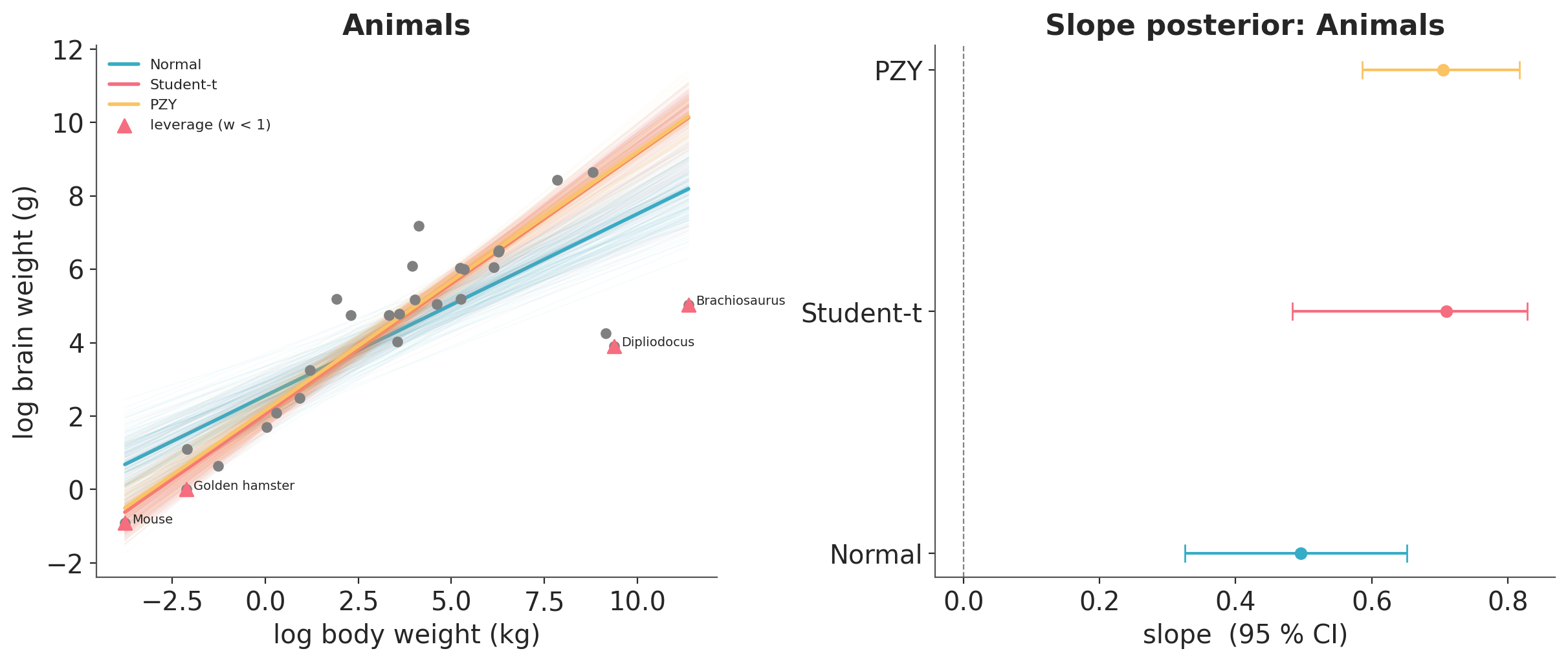
Dataset 1: brain and body weights#
The Animals dataset from Venables and Ripley [2002] has body weight (kg) and
brain weight (g) for 28 species. On a log-log scale the relationship is
roughly linear, except for a handful of species at the extremes: dinosaurs at
the top end (very large body, small brain relative to body) and the smallest
rodents at the bottom end. The Normal and Student-t fits are pulled toward
those points. PZY downweights them and recovers a steeper slope, close to
the slope you would estimate from the bulk alone.
try:
    animals_df = pd.read_csv(os.path.join("..", "data", "animals.csv"))
except FileNotFoundError:
    animals_df = pd.read_csv("data/animals.csv")

animals_X = np.log(animals_df["body_kg"].values).reshape(-1, 1)
animals_y = np.log(animals_df["brain_g"].values)

animals_normal_idata, animals_normal_model = fit_normal(
    animals_X, animals_y, predictor_names=["log_body"]
)
animals_studentt_idata, animals_studentt_model = fit_studentt(
    animals_X, animals_y, predictor_names=["log_body"]
)
animals_pzy_idata, animals_pzy_model, animals_weights, animals_info = fit_pzy(
    animals_X, animals_y, predictor_names=["log_body"], k=2.0
)
Multiprocess sampling (4 chains in 4 jobs)
NUTS: [intercept, beta, sigma]
Sampling 4 chains for 2_000 tune and 2_000 draw iterations (8_000 + 8_000 draws total) took 2 seconds.
Multiprocess sampling (4 chains in 4 jobs)
NUTS: [intercept, beta, sigma, nu]
Sampling 4 chains for 2_000 tune and 2_000 draw iterations (8_000 + 8_000 draws total) took 4 seconds.
The rhat statistic is larger than 1.01 for some parameters. This indicates problems during sampling. See https://arxiv.org/abs/1903.08008 for details
Multiprocess sampling (4 chains in 4 jobs)
NUTS: [intercept, beta, sigma]
Sampling 4 chains for 2_000 tune and 2_000 draw iterations (8_000 + 8_000 draws total) took 4 seconds.
_plot_dataset(
    animals_X[:, 0],
    animals_y,
    {"Normal": animals_normal_idata, "Student-t": animals_studentt_idata, "PZY": animals_pzy_idata},
    pred="log_body",
    weights=animals_weights,
    df_labels=animals_df["species"],
    xlabel="log body weight (kg)",
    ylabel="log brain weight (g)",
    title="Animals",
)

print("Animals: slope 95 % CI (this notebook vs paper Table 1)")
paper_animals = {"Normal": (0.33, 0.66), "PZY": (0.67, 0.83)}
for name, idata in [
    ("Normal", animals_normal_idata),
    ("Student-t", animals_studentt_idata),
    ("PZY", animals_pzy_idata),
]:
    mean, lo, hi = _slope_hdi(idata, "log_body")
    paper = paper_animals.get(name)
    paper_str = f"  paper=({paper[0]:.2f}, {paper[1]:.2f})" if paper else ""
    print(f"  {name:12s}  mean={mean:.3f}  ours=({lo:.3f}, {hi:.3f}){paper_str}")
Animals: slope 95 % CI (this notebook vs paper Table 1)
  Normal        mean=0.496  ours=(0.326, 0.652)  paper=(0.33, 0.66)
  Student-t     mean=0.710  ours=(0.483, 0.828)
  PZY           mean=0.705  ours=(0.586, 0.817)  paper=(0.67, 0.83)
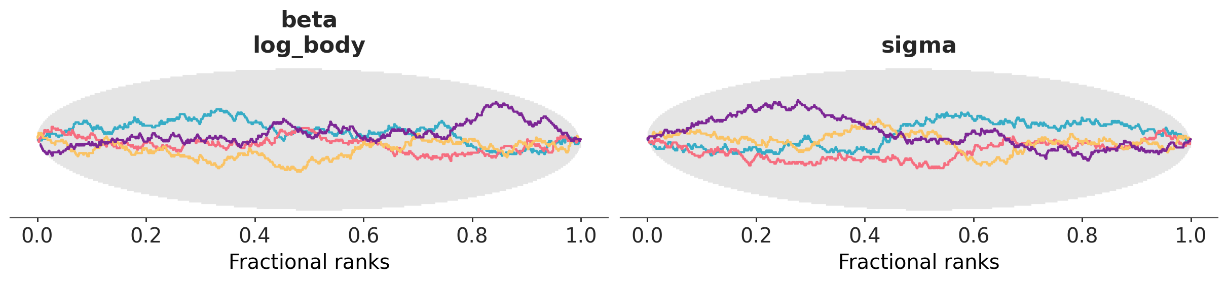
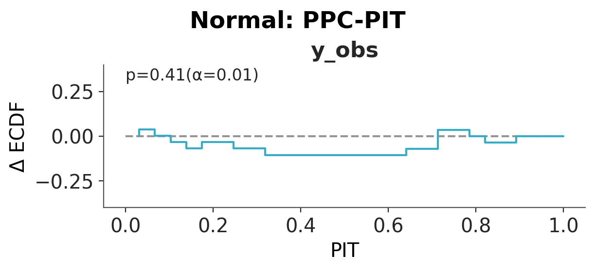
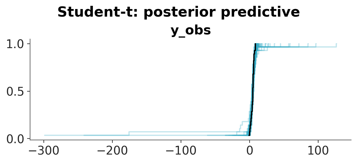
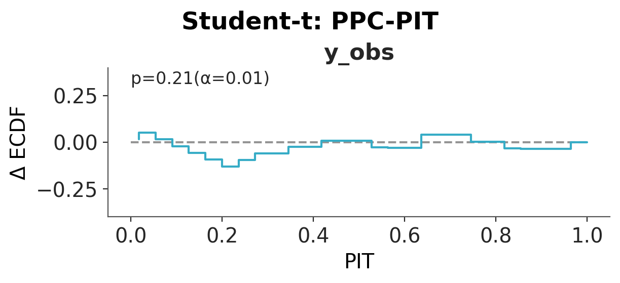
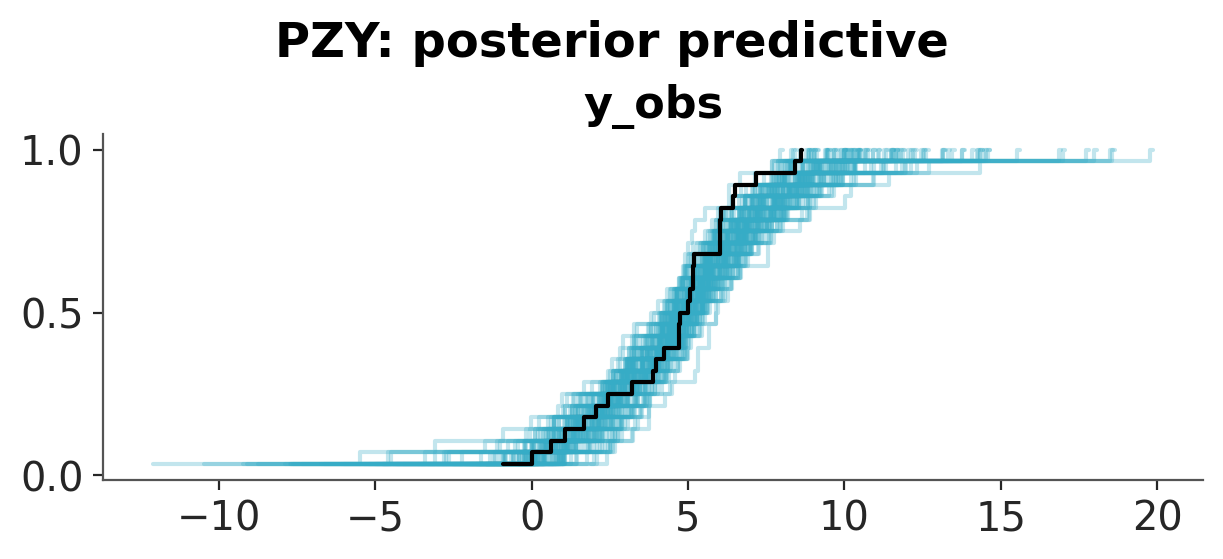
Convergence and posterior predictive checks#
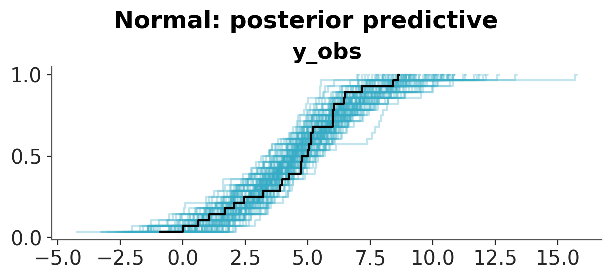
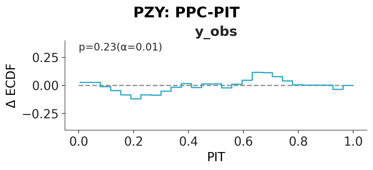
We first check the PZY chains for convergence (see the ArviZ MCMC diagnostics chapter for guidance on \(\hat{R}\) and ESS). Then for each model we draw replicated datasets and a posterior predictive PIT plot. The Normal predictive distribution is too narrow to cover the extreme species. The Student-t covers them by giving every observation heavy tails. PZY covers them by inflating the noise scale only at the downweighted points. A well-calibrated model produces PPC-PIT values close to uniform.
print(
    az.summary(animals_pzy_idata, var_names=["intercept", "beta", "sigma"])[
        ["mean", "sd", "ess_bulk", "ess_tail", "r_hat"]
    ]
)
az.plot_rank(animals_pzy_idata, var_names=["beta", "sigma"])

animals_models = {
    "Normal": animals_normal_model,
    "Student-t": animals_studentt_model,
    "PZY": animals_pzy_model,
}
animals_idatas = {
    "Normal": animals_normal_idata,
    "Student-t": animals_studentt_idata,
    "PZY": animals_pzy_idata,
}
animals_ppcs = {}
for name, model in animals_models.items():
    with model:
        animals_ppcs[name] = pm.sample_posterior_predictive(
            animals_idatas[name], random_seed=RANDOM_SEED, progressbar=False
        )
        # merge posterior_predictive into the inference data tree
        animals_idatas[name]["posterior_predictive"] = animals_ppcs[name]["posterior_predictive"]

for name, idata in animals_idatas.items():
    pc = az.plot_ppc_dist(idata, num_samples=100)
    pc.add_title(f"{name}: posterior predictive")
    pc = az.plot_ppc_pit(idata)
    pc.add_title(f"{name}: PPC-PIT")
                 mean     sd  ess_bulk  ess_tail r_hat
intercept        2.15  0.292      2378      3602  1.00
beta[log_body]  0.705   0.06      2314      3218  1.00
sigma           0.855  0.175      3660      3652  1.00
Sampling: [y_obs]
Sampling: [y_obs]
Sampling: [y_obs]
Dataset 2: CYG OB1 star cluster#
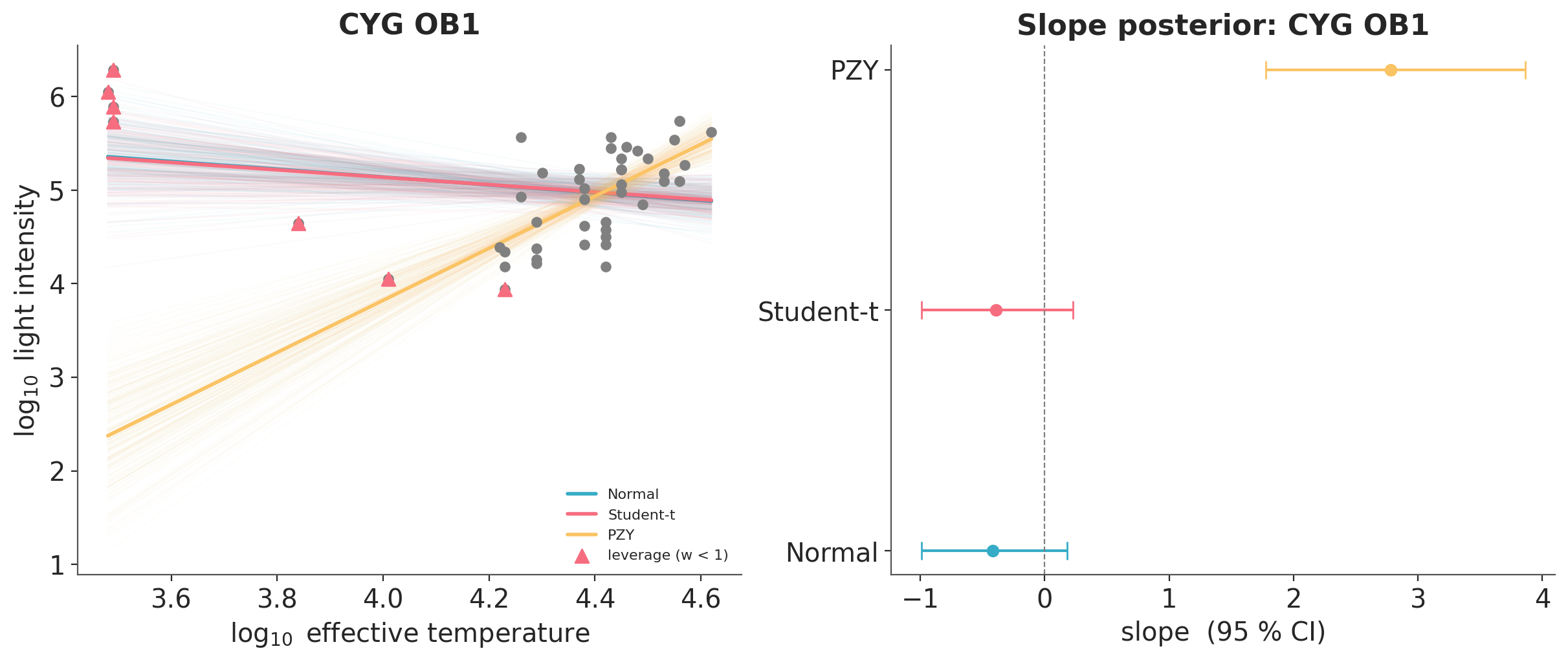
Rousseeuw and Leroy [2005] use the Hertzsprung-Russell diagram for 47 stars in the CYG OB1 cluster [Humphreys, 1978]. The predictor is \(\log_{10}\) effective temperature, and the response is \(\log_{10}\) light intensity. Four giant stars sit apart from the rest: they are cool (low \(\log_{10} T_e\)) but very bright (high \(\log_{10} L\)). These four points pull ordinary regression to a negative slope, the opposite of the expected main-sequence pattern (hotter stars are brighter). PZY downweights the giants and recovers a positive slope.
try:
    cyg_df = pd.read_csv(os.path.join("..", "data", "stars_cyg.csv"))
except FileNotFoundError:
    cyg_df = pd.read_csv("data/stars_cyg.csv")

cyg_X = cyg_df["log.Te"].values.reshape(-1, 1)
cyg_y = cyg_df["log.light"].values

cyg_normal_idata, _ = fit_normal(cyg_X, cyg_y, predictor_names=["log_Te"])
cyg_studentt_idata, _ = fit_studentt(cyg_X, cyg_y, predictor_names=["log_Te"])
cyg_pzy_idata, _, cyg_weights, cyg_info = fit_pzy(cyg_X, cyg_y, predictor_names=["log_Te"], k=2.0)
Multiprocess sampling (4 chains in 4 jobs)
NUTS: [intercept, beta, sigma]
Sampling 4 chains for 2_000 tune and 2_000 draw iterations (8_000 + 8_000 draws total) took 7 seconds.
Multiprocess sampling (4 chains in 4 jobs)
NUTS: [intercept, beta, sigma, nu]
Sampling 4 chains for 2_000 tune and 2_000 draw iterations (8_000 + 8_000 draws total) took 13 seconds.
Multiprocess sampling (4 chains in 4 jobs)
NUTS: [intercept, beta, sigma]
Sampling 4 chains for 2_000 tune and 2_000 draw iterations (8_000 + 8_000 draws total) took 82 seconds.
_plot_dataset(
    cyg_X[:, 0],
    cyg_y,
    {"Normal": cyg_normal_idata, "Student-t": cyg_studentt_idata, "PZY": cyg_pzy_idata},
    pred="log_Te",
    weights=cyg_weights,
    xlabel="$\\log_{10}$ effective temperature",
    ylabel="$\\log_{10}$ light intensity",
    title="CYG OB1",
)

print("CYG OB1: slope 95 % CI (this notebook vs paper Table 2)")
paper_cyg = {"Normal": (-1.00, 0.15), "PZY": (1.96, 3.98)}
for name, idata in [
    ("Normal", cyg_normal_idata),
    ("Student-t", cyg_studentt_idata),
    ("PZY", cyg_pzy_idata),
]:
    mean, lo, hi = _slope_hdi(idata, "log_Te")
    paper = paper_cyg.get(name)
    paper_str = f"  paper=({paper[0]:.2f}, {paper[1]:.2f})" if paper else ""
    print(f"  {name:12s}  mean={mean:.3f}  ours=({lo:.3f}, {hi:.3f}){paper_str}")
CYG OB1: slope 95 % CI (this notebook vs paper Table 2)
  Normal        mean=-0.418  ours=(-0.988, 0.182)  paper=(-1.00, 0.15)
  Student-t     mean=-0.395  ours=(-0.991, 0.225)
  PZY           mean=2.783  ours=(1.777, 3.861)  paper=(1.96, 3.98)
Dataset 3: Hawkins-Bradu-Kass#
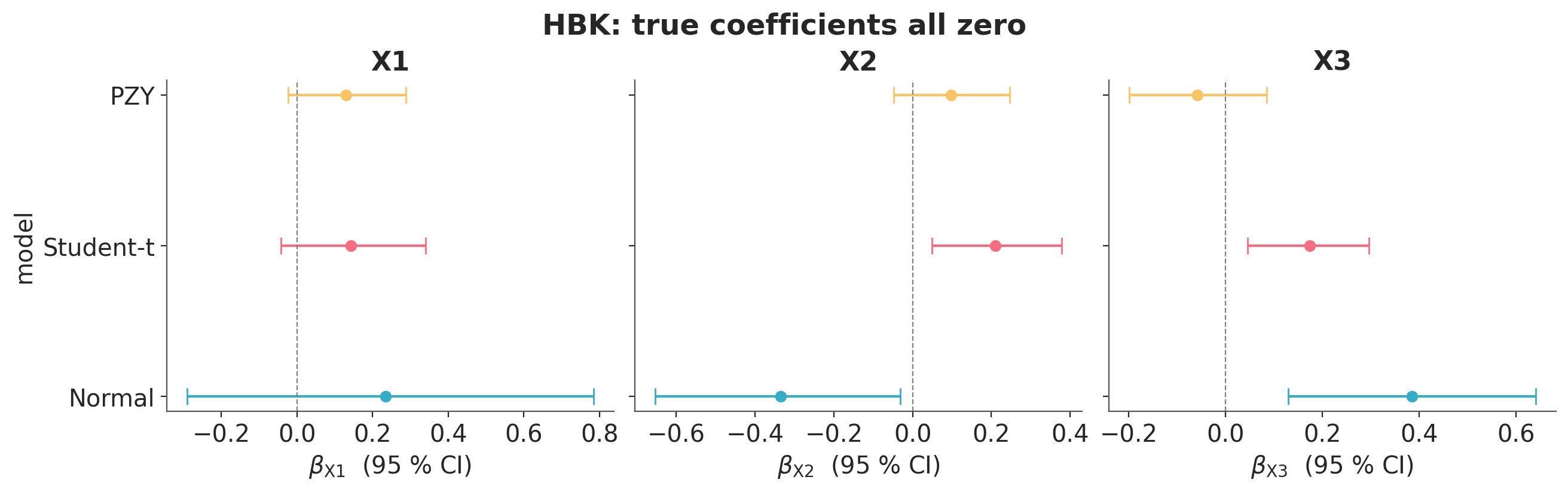
The Hawkins et al. [1984] dataset has 75 observations on three predictors, designed so that the first 14 rows are leverage points: the first 10 have large predictor values and large response values (bad leverage), and rows 11-14 have large predictor values but response near zero (good leverage, consistent with the bulk pattern). The remaining 61 observations cluster near the origin. The true regression coefficients for the bulk are all zero. The Normal and Student-t likelihoods are pulled by the 10 bad leverage points. PZY downweights all 14 leverage points and recovers slopes whose 95 % CIs include zero.
try:
    hbk_df = pd.read_csv(os.path.join("..", "data", "hbk.csv"))
except FileNotFoundError:
    hbk_df = pd.read_csv("data/hbk.csv")

hbk_X = hbk_df[["X1", "X2", "X3"]].values
hbk_y = hbk_df["Y"].values

hbk_normal_idata, _ = fit_normal(hbk_X, hbk_y, predictor_names=["X1", "X2", "X3"])
hbk_studentt_idata, _ = fit_studentt(hbk_X, hbk_y, predictor_names=["X1", "X2", "X3"])
hbk_pzy_idata, _, hbk_weights, hbk_info = fit_pzy(
    hbk_X, hbk_y, predictor_names=["X1", "X2", "X3"], k=2.0
)
Multiprocess sampling (4 chains in 4 jobs)
NUTS: [intercept, beta, sigma]
Sampling 4 chains for 2_000 tune and 2_000 draw iterations (8_000 + 8_000 draws total) took 5 seconds.
Multiprocess sampling (4 chains in 4 jobs)
NUTS: [intercept, beta, sigma, nu]
Sampling 4 chains for 2_000 tune and 2_000 draw iterations (8_000 + 8_000 draws total) took 11 seconds.
Multiprocess sampling (4 chains in 4 jobs)
NUTS: [intercept, beta, sigma]
Sampling 4 chains for 2_000 tune and 2_000 draw iterations (8_000 + 8_000 draws total) took 9 seconds.
fig, axes = plt.subplots(1, 3, figsize=(13, 4), sharey=True)
colors = {"Normal": "C0", "Student-t": "C1", "PZY": "C2"}

for ax, pred in zip(axes, ["X1", "X2", "X3"]):
    for i, (name, idata) in enumerate(
        [("Normal", hbk_normal_idata), ("Student-t", hbk_studentt_idata), ("PZY", hbk_pzy_idata)]
    ):
        mean, lo, hi = _slope_hdi(idata, pred)
        ax.errorbar(
            mean, i, xerr=[[mean - lo], [hi - mean]], fmt="o", color=colors[name], capsize=5
        )
    ax.set_yticks([0, 1, 2])
    ax.set_yticklabels(["Normal", "Student-t", "PZY"])
    ax.axvline(0, color="gray", ls="--", lw=0.8)
    ax.set_xlabel(f"$\\beta_{{\\text{{{pred}}}}}$  (95 % CI)")
    ax.set_title(pred)

axes[0].set_ylabel("model")
fig.suptitle("HBK: true coefficients all zero")

print("HBK: coefficient 95 % CIs (true values: all zero)")
print(f"{'Model':12s}  {'X1':>18s}  {'X2':>18s}  {'X3':>18s}")
for name, idata in [
    ("Normal", hbk_normal_idata),
    ("Student-t", hbk_studentt_idata),
    ("PZY", hbk_pzy_idata),
]:
    row = []
    for pred in ["X1", "X2", "X3"]:
        mean, lo, hi = _slope_hdi(idata, pred)
        row.append(f"{mean:+.2f} ({lo:+.2f}, {hi:+.2f})")
    print(f"  {name:12s}  {'  '.join(row)}")
print("Paper Table 3 PZY:    " "+0.06 (-0.06, +0.19)  +0.02 (-0.11, +0.14)  -0.12 (-0.24, +0.01)")
HBK: coefficient 95 % CIs (true values: all zero)
Model                         X1                  X2                  X3
  Normal        +0.23 (-0.29, +0.79)  -0.34 (-0.65, -0.03)  +0.39 (+0.13, +0.64)
  Student-t     +0.14 (-0.04, +0.34)  +0.21 (+0.05, +0.38)  +0.17 (+0.05, +0.30)
  PZY           +0.13 (-0.02, +0.29)  +0.10 (-0.05, +0.25)  -0.06 (-0.20, +0.08)
Paper Table 3 PZY:    +0.06 (-0.06, +0.19)  +0.02 (-0.11, +0.14)  -0.12 (-0.24, +0.01)
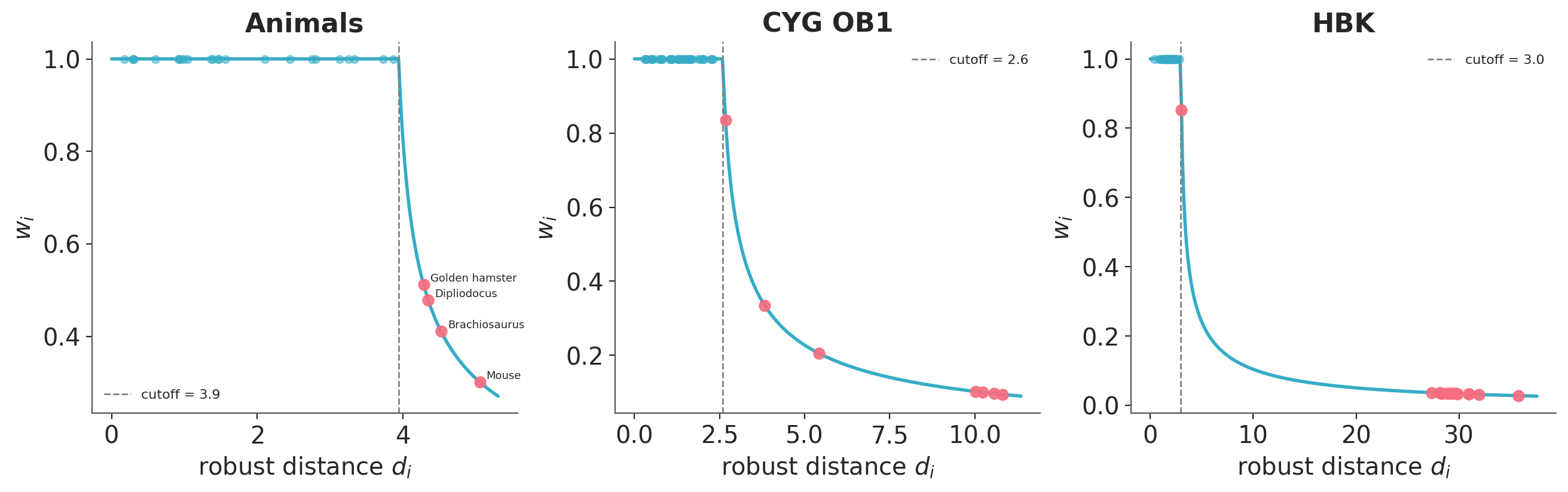
Weights across datasets#
The plot below shows each observation’s PZY weight against its robust Mahalanobis distance, for all three datasets. Points left of the dashed cutoff line have weight 1. Points to the right are downweighted smoothly, with weight decreasing as the distance grows.
fig, axes = plt.subplots(1, 3, figsize=(13, 4))
datasets = [
    ("Animals", animals_info, animals_weights, animals_df["species"]),
    ("CYG OB1", cyg_info, cyg_weights, None),
    ("HBK", hbk_info, hbk_weights, None),
]
for ax, (title, info, weights, labels) in zip(axes, datasets):
    d, a = info["distances"], info["cutoff"]
    d_plot = np.linspace(0, d.max() * 1.05, 300)
    w_plot = np.where(d_plot <= a, 1.0, 1.0 / np.sqrt(np.maximum(1.0, 1 + d_plot**2 - a**2)))
    ax.plot(d_plot, w_plot, color="C0", lw=2, zorder=2)
    ax.axvline(a, color="gray", ls="--", lw=1, label=f"cutoff = {a:.1f}")
    mask = weights < 1.0
    ax.scatter(d[~mask], weights[~mask], color="C0", alpha=0.5, s=20, zorder=3)
    ax.scatter(d[mask], weights[mask], color="C1", alpha=0.9, s=40, zorder=4)
    if labels is not None:
        for i in np.where(mask)[0]:
            ax.annotate(
                labels.iloc[i],
                (d[i], weights[i]),
                fontsize=6.5,
                xytext=(4, 2),
                textcoords="offset points",
            )
    ax.set_xlabel("robust distance $d_i$")
    ax.set_ylabel("$w_i$")
    ax.set_title(title)
    ax.legend(fontsize=8)
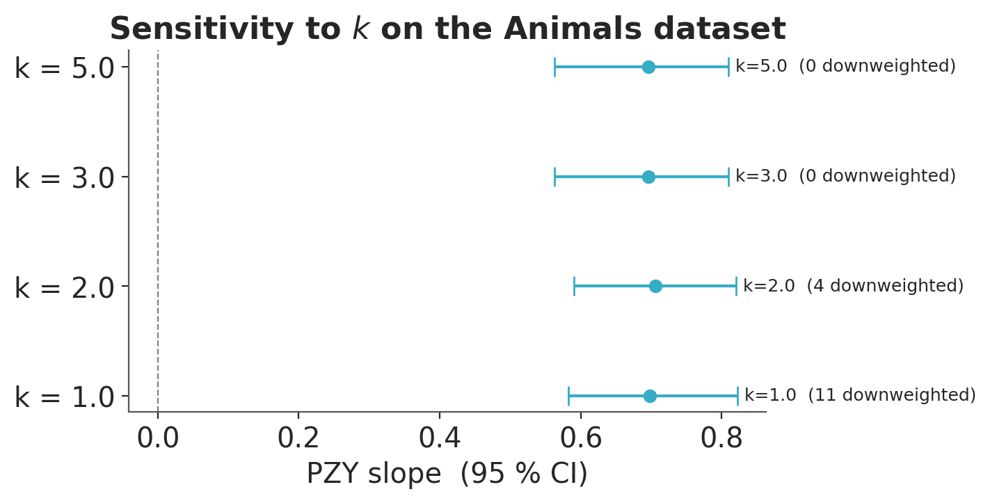
Sensitivity to the tuning parameter \(k\)#
The cutoff \(a = \text{median}(d) + k \cdot \text{MAD}(d)\) is controlled by \(k\). A small \(k\) is aggressive (more observations downweighted); a large \(k\) is conservative. We vary \(k \in \{1, 2, 3, 5\}\) on the Animals dataset and compare the resulting slope posteriors.
k_values = [1.0, 2.0, 3.0, 5.0]
k_results = {}

for k_val in k_values:
    idata_k, _, weights_k, _ = fit_pzy(
        animals_X,
        animals_y,
        predictor_names=["log_body"],
        k=k_val,
        draws=1000,
        tune=1000,
    )
    mean, lo, hi = _slope_hdi(idata_k, "log_body")
    k_results[k_val] = (mean, lo, hi, int((weights_k < 1).sum()))

fig, ax = plt.subplots(figsize=(7, 3.5))
for i, k_val in enumerate(k_values):
    mean, lo, hi, n_down = k_results[k_val]
    ax.errorbar(mean, i, xerr=[[mean - lo], [hi - mean]], fmt="o", color="C0", capsize=5)
    ax.text(hi + 0.01, i, f"k={k_val}  ({n_down} downweighted)", va="center", fontsize=9)
ax.set_yticks(range(len(k_values)))
ax.set_yticklabels([f"k = {k}" for k in k_values])
ax.set_xlabel("PZY slope  (95 % CI)")
ax.set_title("Sensitivity to $k$ on the Animals dataset")
ax.axvline(0, color="gray", ls="--", lw=0.8)
Multiprocess sampling (4 chains in 4 jobs)
NUTS: [intercept, beta, sigma]
Sampling 4 chains for 1_000 tune and 1_000 draw iterations (4_000 + 4_000 draws total) took 3 seconds.
Multiprocess sampling (4 chains in 4 jobs)
NUTS: [intercept, beta, sigma]
Sampling 4 chains for 1_000 tune and 1_000 draw iterations (4_000 + 4_000 draws total) took 2 seconds.
Multiprocess sampling (4 chains in 4 jobs)
NUTS: [intercept, beta, sigma]
Sampling 4 chains for 1_000 tune and 1_000 draw iterations (4_000 + 4_000 draws total) took 2 seconds.
Multiprocess sampling (4 chains in 4 jobs)
NUTS: [intercept, beta, sigma]
Sampling 4 chains for 1_000 tune and 1_000 draw iterations (4_000 + 4_000 draws total) took 2 seconds.
<matplotlib.lines.Line2D at 0x7f36a876ca50>
Limitations#
Good leverage points are downweighted too. The distance-based criterion cannot tell a harmful leverage point from a useful one. Extreme but valid observations on the true regression surface still get reduced weight, which widens credible intervals.
Single-cluster assumption. The quadrant correlation estimates a single robust center for the joint distribution of \((y, X)\). If the predictor space has more than one cluster, the algorithm may flag a real secondary cluster as leverage points.
Weights are pre-computed, not sampled. The \(w_i\) are fixed before MCMC starts and do not adapt as the posterior of \(\beta\) is explored. A fully Bayesian treatment would model the weights as random variables, but that is much harder to fit.
Not appropriate for structured data. The i.i.d. error assumption that justifies the quadrant-correlation distance breaks down for hierarchical models, time series, or any other data with dependence between observations.
References#
Daniel Peña, Ruben Zamar, and Guohua Yan. Bayesian likelihood robustness in linear models. Journal of Statistical Planning and Inference, 139(7):2196–2207, 2009. doi:10.1016/j.jspi.2008.10.012.
Peter J. Huber. Robust Statistics. Wiley Series in Probability and Mathematical Statistics. Wiley, New York, 1981.
W. N. Venables and B. D. Ripley. Modern Applied Statistics with S. Springer, New York, 4 edition, 2002. ISBN 0-387-95457-0.
Peter J. Rousseeuw and Annick M. Leroy. Robust Regression and Outlier Detection. Wiley, Hoboken, NJ, 2005. ISBN 978-0-471-48855-2.
Roberta M. Humphreys. Studies of luminous stars in nearby galaxies. I. supergiants and O stars in the Milky Way. Astrophysical Journal Supplement Series, 38:309–350, 1978. doi:10.1086/190559.
Douglas M. Hawkins, Dan Bradu, and Gordon V. Kass. Location of several outliers in multiple-regression data using elemental sets. Technometrics, 26(3):197–208, 1984. doi:10.1080/00401706.1984.10487956.
%load_ext watermark
%watermark -n -u -v -iv -w -p pytensor,xarray
Last updated: Tue, 12 May 2026

Python implementation: CPython
Python version       : 3.13.12
IPython version      : 9.13.0

pytensor: 3.0.1
xarray  : 2026.4.0

arviz     : 1.1.0
matplotlib: 3.10.9
numpy     : 2.4.4
pandas    : 3.0.2
pymc      : 5.28.0+87.g9491f60db

Watermark: 2.6.0
License notice#
All the notebooks in this example gallery are provided under the MIT License which allows modification, and redistribution for any use provided the copyright and license notices are preserved.
Citing PyMC examples#
To cite this notebook, use the DOI provided by Zenodo for the pymc-examples repository.
Important
Many notebooks are adapted from other sources: blogs, books… In such cases you should cite the original source as well.
Also remember to cite the relevant libraries used by your code.
Here is an citation template in bibtex:
@incollection{citekey,
  author    = "<notebook authors, see above>",
  title     = "<notebook title>",
  editor    = "PyMC Team",
  booktitle = "PyMC examples",
  doi       = "10.5281/zenodo.5654871"
}
which once rendered could look like: