GLM: Negative Binomial Regression

Attention

This notebook uses libraries that are not PyMC dependencies and therefore need to be installed specifically to run this notebook. Open the dropdown below for extra guidance.

Extra dependencies install instructions

In order to run this notebook (either locally or on binder) you won’t only need a working PyMC installation with all optional dependencies, but also to install some extra dependencies. For advise on installing PyMC itself, please refer to Installation

You can install these dependencies with your preferred package manager, we provide as an example the pip and conda commands below.

$ pip install seaborn

Note that if you want (or need) to install the packages from inside the notebook instead of the command line, you can install the packages by running a variation of the pip command:

import sys

!{sys.executable} -m pip install seaborn

You should not run !pip install as it might install the package in a different environment and not be available from the Jupyter notebook even if installed.

Another alternative is using conda instead:

$ conda install seaborn

when installing scientific python packages with conda, we recommend using conda forge

import arviz as az
import numpy as np
import pandas as pd
import pymc as pm
import seaborn as sns

from scipy import stats

RANDOM_SEED = 8927
rng = np.random.default_rng(RANDOM_SEED)

%config InlineBackend.figure_format = "retina"
az.style.use("arviz-darkgrid")

This notebook closely follows the GLM Poisson regression example by Jonathan Sedar (which is in turn inspired by a project by Ian Osvald) except the data here is negative binomially distributed instead of Poisson distributed.

Negative binomial regression is used to model count data for which the variance is higher than the mean. The negative binomial distribution can be thought of as a Poisson distribution whose rate parameter is gamma distributed, so that rate parameter can be adjusted to account for the increased variance.

Generate Data

As in the Poisson regression example, we assume that sneezing occurs at some baseline rate, and that consuming alcohol, not taking antihistamines, or doing both, increase its frequency.

Poisson Data

First, let’s look at some Poisson distributed data from the Poisson regression example.

# Mean Poisson values
theta_noalcohol_meds = 1  # no alcohol, took an antihist
theta_alcohol_meds = 3  # alcohol, took an antihist
theta_noalcohol_nomeds = 6  # no alcohol, no antihist
theta_alcohol_nomeds = 36  # alcohol, no antihist

# Create samples
q = 1000
df_pois = pd.DataFrame(
    {
        "nsneeze": np.concatenate(
            (
                rng.poisson(theta_noalcohol_meds, q),
                rng.poisson(theta_alcohol_meds, q),
                rng.poisson(theta_noalcohol_nomeds, q),
                rng.poisson(theta_alcohol_nomeds, q),
            )
        ),
        "alcohol": np.concatenate(
            (
                np.repeat(False, q),
                np.repeat(True, q),
                np.repeat(False, q),
                np.repeat(True, q),
            )
        ),
        "nomeds": np.concatenate(
            (
                np.repeat(False, q),
                np.repeat(False, q),
                np.repeat(True, q),
                np.repeat(True, q),
            )
        ),
    }
)

df_pois.groupby(["nomeds", "alcohol"])["nsneeze"].agg(["mean", "var"])

		mean	var
nomeds	alcohol
False	False	1.047	1.127919
	True	2.986	2.960765
True	False	5.981	6.218858
	True	35.929	36.064023

Since the mean and variance of a Poisson distributed random variable are equal, the sample means and variances are very close.

Negative Binomial Data

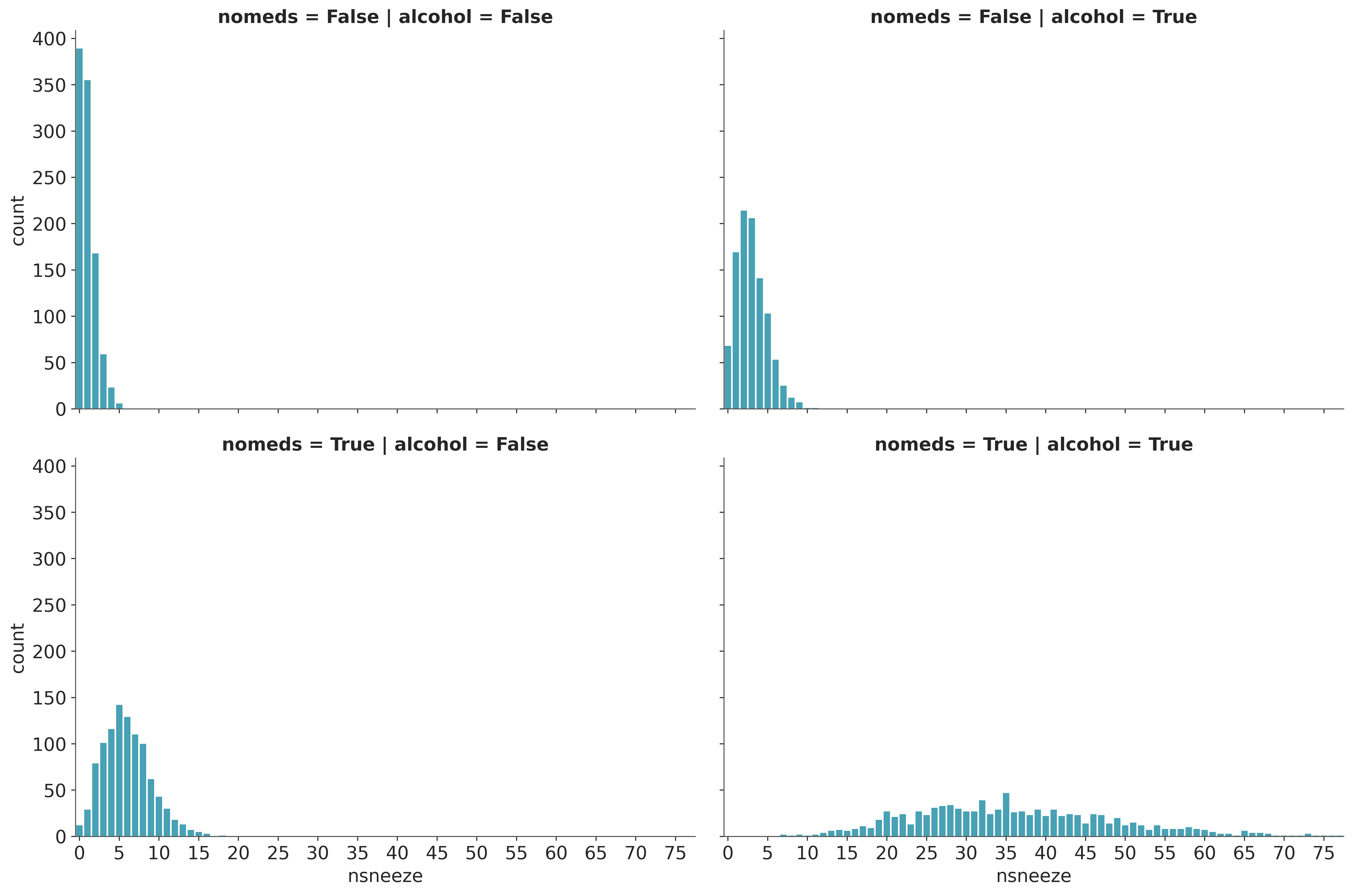
Now, suppose every subject in the dataset had the flu, increasing the variance of their sneezing (and causing an unfortunate few to sneeze over 70 times a day). If the mean number of sneezes stays the same but variance increases, the data might follow a negative binomial distribution.

# Gamma shape parameter
alpha = 10


def get_nb_vals(mu, alpha, size):
    """Generate negative binomially distributed samples by
    drawing a sample from a gamma distribution with mean `mu` and
    shape parameter `alpha', then drawing from a Poisson
    distribution whose rate parameter is given by the sampled
    gamma variable.

    """

    g = stats.gamma.rvs(alpha, scale=mu / alpha, size=size)
    return stats.poisson.rvs(g)


# Create samples
n = 1000
df = pd.DataFrame(
    {
        "nsneeze": np.concatenate(
            (
                get_nb_vals(theta_noalcohol_meds, alpha, n),
                get_nb_vals(theta_alcohol_meds, alpha, n),
                get_nb_vals(theta_noalcohol_nomeds, alpha, n),
                get_nb_vals(theta_alcohol_nomeds, alpha, n),
            )
        ),
        "alcohol": np.concatenate(
            (
                np.repeat(False, n),
                np.repeat(True, n),
                np.repeat(False, n),
                np.repeat(True, n),
            )
        ),
        "nomeds": np.concatenate(
            (
                np.repeat(False, n),
                np.repeat(False, n),
                np.repeat(True, n),
                np.repeat(True, n),
            )
        ),
    }
)
df

	nsneeze	alcohol	nomeds
0	2	False	False
1	1	False	False
2	2	False	False
3	2	False	False
4	3	False	False
...	...	...	...
3995	28	True	True
3996	63	True	True
3997	19	True	True
3998	34	True	True
3999	40	True	True

4000 rows × 3 columns

df.groupby(["nomeds", "alcohol"])["nsneeze"].agg(["mean", "var"])

		mean	var
nomeds	alcohol
False	False	0.990	1.137037
	True	2.983	4.030742
True	False	6.004	8.658643
	True	35.918	169.018294

As in the Poisson regression example, we see that drinking alcohol and/or not taking antihistamines increase the sneezing rate to varying degrees. Unlike in that example, for each combination of alcohol and nomeds, the variance of nsneeze is higher than the mean. This suggests that a Poisson distribution would be a poor fit for the data since the mean and variance of a Poisson distribution are equal.

Visualize the Data

g = sns.catplot(x="nsneeze", row="nomeds", col="alcohol", data=df, kind="count", aspect=1.5)

# Make x-axis ticklabels less crowded
ax = g.axes[1, 0]
labels = range(len(ax.get_xticklabels(which="both")))
ax.set_xticks(labels[::5])
ax.set_xticklabels(labels[::5]);

/opt/homebrew/Caskroom/miniconda/base/envs/pymc-dev/lib/python3.11/site-packages/seaborn/axisgrid.py:123: UserWarning: The figure layout has changed to tight
  self._figure.tight_layout(*args, **kwargs)
/opt/homebrew/Caskroom/miniconda/base/envs/pymc-dev/lib/python3.11/site-packages/seaborn/axisgrid.py:123: UserWarning: The figure layout has changed to tight
  self._figure.tight_layout(*args, **kwargs)

Negative Binomial Regression

Create GLM Model

COORDS = {"regressor": ["nomeds", "alcohol", "nomeds:alcohol"], "obs_idx": df.index}

with pm.Model(coords=COORDS) as m_sneeze_inter:
    a = pm.Normal("intercept", mu=0, sigma=5)
    b = pm.Normal("slopes", mu=0, sigma=1, dims="regressor")
    alpha = pm.Exponential("alpha", 0.5)

    M = pm.ConstantData("nomeds", df.nomeds.to_numpy(), dims="obs_idx")
    A = pm.ConstantData("alcohol", df.alcohol.to_numpy(), dims="obs_idx")
    S = pm.ConstantData("nsneeze", df.nsneeze.to_numpy(), dims="obs_idx")

    λ = pm.math.exp(a + b[0] * M + b[1] * A + b[2] * M * A)

    y = pm.NegativeBinomial("y", mu=λ, alpha=alpha, observed=S, dims="obs_idx")

    idata = pm.sample()

Auto-assigning NUTS sampler...
Initializing NUTS using jitter+adapt_diag...
Multiprocess sampling (4 chains in 4 jobs)
NUTS: [intercept, slopes, alpha]

100.00% [8000/8000 00:10<00:00 Sampling 4 chains, 0 divergences]

Sampling 4 chains for 1_000 tune and 1_000 draw iterations (4_000 + 4_000 draws total) took 11 seconds.

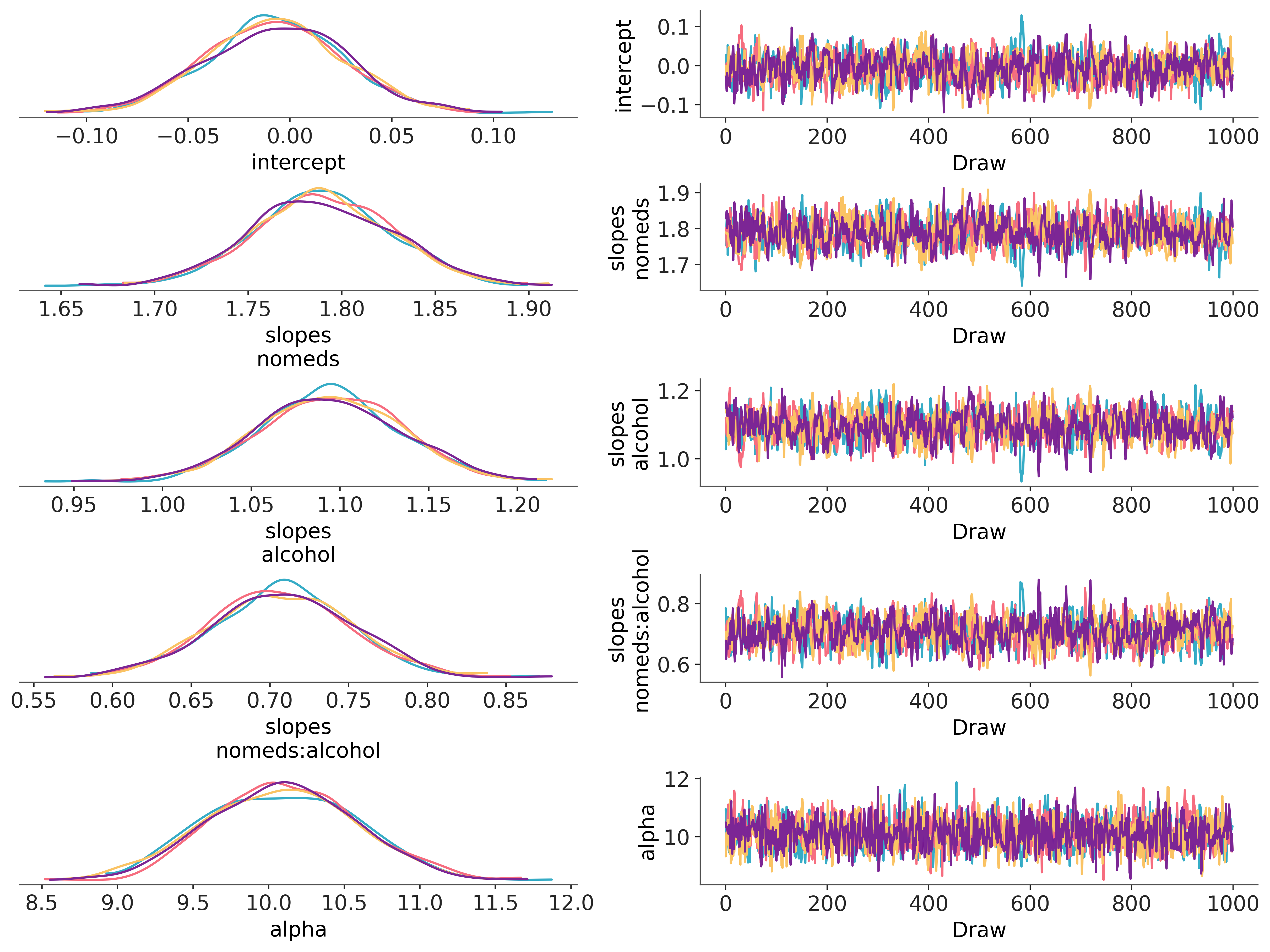
View Results

az.plot_trace(idata, compact=False);

# Transform coefficients to recover parameter values
az.summary(np.exp(idata.posterior), kind="stats", var_names=["intercept", "slopes"])

	mean	sd	hdi_3%	hdi_97%
intercept	0.993	0.033	0.935	1.056
slopes[nomeds]	6.048	0.221	5.635	6.438
slopes[alcohol]	3.006	0.115	2.789	3.215
slopes[nomeds:alcohol]	1.995	0.086	1.842	2.163

az.summary(idata.posterior, kind="stats", var_names="alpha")

	mean	sd	hdi_3%	hdi_97%
alpha	9.909	0.487	9.05	10.887

The mean values are close to the values we specified when generating the data:

• The base rate is a constant 1.

• Drinking alcohol triples the base rate.

• Not taking antihistamines increases the base rate by 6 times.

• Drinking alcohol and not taking antihistamines doubles the rate that would be expected if their rates were independent. If they were independent, then doing both would increase the base rate by 3*6=18 times, but instead the base rate is increased by 3*6*2=36 times.

Finally, the mean of nsneeze_alpha is also quite close to its actual value of 10.

See also, bambi's negative binomial example for further reference.

Authors

• Created by Ian Ozsvald

• Updated by Abhipsha Das in August 2021

• Updated by Benjamin Vincent to PyMC v4 in June 2022

• Updated by Wesley Boelrijk to PyMC v5 in September 2023

%load_ext watermark
%watermark -n -u -v -iv -w -p pytensor,xarray

Last updated: Mon Oct 16 2023

Python implementation: CPython
Python version       : 3.11.5
IPython version      : 8.15.0

pytensor: 2.16.1
xarray  : 2023.8.0

pymc   : 5.8.1
pandas : 2.1.0
seaborn: 0.13.0
numpy  : 1.25.2
arviz  : 0.16.1
scipy  : 1.11.2

Watermark: 2.4.3

License notice

All the notebooks in this example gallery are provided under the MIT License which allows modification, and redistribution for any use provided the copyright and license notices are preserved.

Citing PyMC examples

To cite this notebook, use the DOI provided by Zenodo for the pymc-examples repository.

Important

Many notebooks are adapted from other sources: blogs, books… In such cases you should cite the original source as well.

Also remember to cite the relevant libraries used by your code.

Here is an citation template in bibtex:

@incollection{citekey,
  author    = "<notebook authors, see above>",
  title     = "<notebook title>",
  editor    = "PyMC Team",
  booktitle = "PyMC examples",
  doi       = "10.5281/zenodo.5654871"
}

which once rendered could look like: