


Gaussian Processes using numpy kernel#
Example of simple Gaussian Process fit, adapted from Stan’s example-models repository.
For illustrative and divulgative purposes, this example builds a Gaussian process from scratch. However, PyMC includes a module dedicated to Gaussian Processes which is recommended instead of coding everything from scratch.
import arviz as az
import matplotlib.pyplot as plt
import numpy as np
import pymc as pm
import pytensor.tensor as pt
import seaborn as sns

from xarray_einstats.stats import multivariate_normal

print(f"Running on PyMC v{pm.__version__}")
Running on PyMC v4.1.3
RANDOM_SEED = 8927
rng = np.random.default_rng(RANDOM_SEED)
az.style.use("arviz-darkgrid")
# fmt: off
x = np.array([-5, -4.9, -4.8, -4.7, -4.6, -4.5, -4.4, -4.3, -4.2, -4.1, -4,
-3.9, -3.8, -3.7, -3.6, -3.5, -3.4, -3.3, -3.2, -3.1, -3, -2.9,
-2.8, -2.7, -2.6, -2.5, -2.4, -2.3, -2.2, -2.1, -2, -1.9, -1.8,
-1.7, -1.6, -1.5, -1.4, -1.3, -1.2, -1.1, -1, -0.9, -0.8, -0.7,
-0.6, -0.5, -0.4, -0.3, -0.2, -0.1, 0, 0.1, 0.2, 0.3, 0.4, 0.5,
0.6, 0.7, 0.8, 0.9, 1, 1.1, 1.2, 1.3, 1.4, 1.5, 1.6, 1.7, 1.8,
1.9, 2, 2.1, 2.2, 2.3, 2.4, 2.5, 2.6, 2.7, 2.8, 2.9, 3, 3.1,
3.2, 3.3, 3.4, 3.5, 3.6, 3.7, 3.8, 3.9, 4, 4.1, 4.2, 4.3, 4.4,
4.5, 4.6, 4.7, 4.8, 4.9, 5])

y = np.array([1.04442478194401, 0.948306088493654, 0.357037759697332, 0.492336514646604,
0.520651364364746, 0.112629866592809, 0.470995468454158, -0.168442254267804,
0.0720344402575861, -0.188108980535916, -0.0160163306512027,
-0.0388792158617705, -0.0600673630622568, 0.113568725264636,
0.447160403837629, 0.664421188556779, -0.139510743820276, 0.458823971660986,
0.141214654640904, -0.286957663528091, -0.466537724021695, -0.308185884317105,
-1.57664872694079, -1.44463024170082, -1.51206214603847, -1.49393593601901,
-2.02292464164487, -1.57047488853653, -1.22973445533419, -1.51502367058357,
-1.41493587255224, -1.10140254663611, -0.591866485375275, -1.08781838696462,
-0.800375653733931, -1.00764767602679, -0.0471028950122742, -0.536820626879737,
-0.151688056391446, -0.176771681318393, -0.240094952335518, -1.16827876746502,
-0.493597351974992, -0.831683011472805, -0.152347043914137, 0.0190364158178343,
-1.09355955218051, -0.328157917911376, -0.585575679802941, -0.472837120425201,
-0.503633622750049, -0.0124446353828312, -0.465529814250314,
-0.101621725887347, -0.26988462590405, 0.398726664193302, 0.113805181040188,
0.331353802465398, 0.383592361618461, 0.431647298655434, 0.580036473774238,
0.830404669466897, 1.17919105883462, 0.871037583886711, 1.12290553424174,
0.752564860804382, 0.76897960270623, 1.14738839410786, 0.773151715269892,
0.700611498974798, 0.0412951045437818, 0.303526087747629, -0.139399513324585,
-0.862987735433697, -1.23399179134008, -1.58924289116396, -1.35105117911049,
-0.990144529089174, -1.91175364127672, -1.31836236129543, -1.65955735224704,
-1.83516148300526, -2.03817062501248, -1.66764011409214, -0.552154350554687,
-0.547807883952654, -0.905389222477036, -0.737156477425302, -0.40211249920415,
0.129669958952991, 0.271142753510592, 0.176311762529962, 0.283580281859344,
0.635808289696458, 1.69976647982837, 1.10748978734239, 0.365412229181044,
0.788821368082444, 0.879731888124867, 1.02180766619069, 0.551526067300283])
# fmt: on
N = len(y)
We will use a squared exponential covariance function, which relies on the squared distances between observed points in the data.
squared_distance = lambda x, y: (x[None, :] - y[:, None]) ** 2
with pm.Model() as gp_fit:
    mu = np.zeros(N)

    eta_sq = pm.HalfCauchy("eta_sq", 5)
    rho_sq = pm.HalfCauchy("rho_sq", 5)
    sigma_sq = pm.HalfCauchy("sigma_sq", 5)

    D = squared_distance(x, x)

    # Squared exponential
    sigma = pt.fill_diagonal(eta_sq * pt.exp(-rho_sq * D), eta_sq + sigma_sq)

    obs = pm.MvNormal("obs", mu, sigma, observed=y)
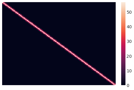
This is what our initial covariance matrix looks like. Intuitively, every data point’s Y-value correlates with points according to their squared distances.
sns.heatmap(sigma.eval(), xticklabels=False, yticklabels=False);
The following generates predictions from the Gaussian Process model in a grid of values:
# Prediction over grid
xgrid = np.linspace(-6, 6)
D_pred = squared_distance(xgrid, xgrid)
D_off_diag = squared_distance(x, xgrid)

gp_fit.add_coords({"pred_id": xgrid, "pred_id2": xgrid})

with gp_fit as gp:
    # Covariance matrices for prediction
    sigma_pred = eta_sq * pt.exp(-rho_sq * D_pred)
    sigma_off_diag = eta_sq * pt.exp(-rho_sq * D_off_diag)

    # Posterior mean
    mu_post = pm.Deterministic(
        "mu_post", pt.dot(pt.dot(sigma_off_diag, pm.math.matrix_inverse(sigma)), y), dims="pred_id"
    )
    # Posterior covariance
    sigma_post = pm.Deterministic(
        "sigma_post",
        sigma_pred
        - pt.dot(pt.dot(sigma_off_diag, pm.math.matrix_inverse(sigma)), sigma_off_diag.T),
        dims=("pred_id", "pred_id2"),
    )
with gp_fit:
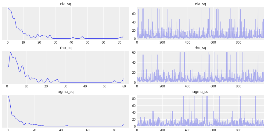
svgd_approx = pm.fit(400, method="svgd", inf_kwargs=dict(n_particles=100))
gp_trace = svgd_approx.sample(1000)
az.plot_trace(gp_trace, var_names=["eta_sq", "rho_sq", "sigma_sq"]);
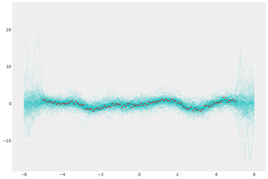
Sample from the posterior Gaussian Process
post = az.extract(gp_trace, num_samples=200)

y_pred = multivariate_normal(
    post["mu_post"], post["sigma_post"], dims=("pred_id", "pred_id2")
).rvs()
_, ax = plt.subplots(figsize=(12, 8))
ax.plot(xgrid, y_pred.transpose(..., "sample"), "c-", alpha=0.1)
ax.plot(x, y, "r.");
Watermark#
%load_ext watermark
%watermark -n -u -v -iv -w -p pytensor,aeppl,xarray,xarray_einstats
Last updated: Tue Aug 02 2022

Python implementation: CPython
Python version       : 3.10.5
IPython version      : 8.4.0

pytensor         : 2.7.7
aeppl          : 0.0.32
xarray         : 2022.6.0
xarray_einstats: 0.4.0.dev1

sys       : 3.10.5 | packaged by conda-forge | (main, Jun 14 2022, 07:07:06) [Clang 13.0.1 ]
pytensor    : 2.7.7
pymc      : 4.1.3
seaborn   : 0.11.2
matplotlib: 3.5.2
arviz     : 0.13.0.dev0
numpy     : 1.23.1

Watermark: 2.3.1
License notice#
All the notebooks in this example gallery are provided under the MIT License which allows modification, and redistribution for any use provided the copyright and license notices are preserved.
Citing PyMC examples#
To cite this notebook, use the DOI provided by Zenodo for the pymc-examples repository.
Important
Many notebooks are adapted from other sources: blogs, books… In such cases you should cite the original source as well.
Also remember to cite the relevant libraries used by your code.
Here is an citation template in bibtex:
@incollection{citekey,
  author    = "<notebook authors, see above>",
  title     = "<notebook title>",
  editor    = "PyMC Team",
  booktitle = "PyMC examples",
  doi       = "10.5281/zenodo.5654871"
}
which once rendered could look like: