Example: Mauna Loa CO\(_2\) continued

This GP example shows how to

• Fit fully Bayesian GPs with NUTS

• Model inputs whose exact locations are uncertain (uncertainty in ‘x’)

• Design a semiparametric Gaussian process model

• Build a changepoint covariance function / kernel

• Definine a custom mean and a custom covariance function

Ice Core Data

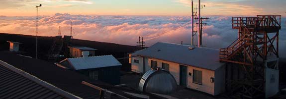
The first data set we’ll look at is CO2 measurements from ice core data. This data goes back to the year 13 AD. The data after the year 1958 is an average of ice core measurements and more accurate data taken from Mauna Loa. I’m very grateful to Tobias Erhardt from the University of Bërn for his generous insight on the science of how some of the processes touched on actually work. Any mistakes are my own of course.

This data is less accurate than the Mauna Loa atmospheric CO2 measurements. Snow that falls on Antarctica accumulates gradually and hardens into ice over time, which is referred to as firn. CO2 measured in the Law Dome ice cores come from air bubbles trapped in the ice. If this ice were flash frozen, the amount of CO2 contained in the air bubbles would reflect the amount of CO2 in the atmosphere at the exact date and time of the freeze. Instead, the process happens gradually, so the trapped air has time to diffuse throughout the solidifying ice. The process of the layering, freezing and solidifying of the firn happens over the scale of years. For the Law Dome data used here, the CO2 measurements listed in the data represent an average CO2 across about 2-4 years in total.

Also, the ordering of the data points is fixed. There is no way for older ice layers to end up on top of newer ice layers. This enforces that we place a prior on the measurement locations whose order is restricted.

The dates of the ice core measurements have some uncertainty. They may be accurate on a yearly level due to how the ice layers on it self every year, but the date isn’t likely to be reliable as to the season when the measurement was taken. Also, the CO2 level observed may be some sort of average of the overall yearly level.

As we saw in the previous example, there is a strong seasonal component in CO2 levels that won’t be observable in this data set. In PyMC3, we can easily include both errors in \(y\) and errors in \(x\). To demonstrate this, we remove the latter part of the data (which are averaged with Mauna Loa readings) so we have only the ice core measurements. We fit the Gaussian process model using the No-U-Turn MCMC sampler.

import arviz as az
import matplotlib.pyplot as plt
import numpy as np
import pandas as pd
import pymc3 as pm
import theano
import theano.tensor as tt

%config InlineBackend.figure_format = 'retina'
RANDOM_SEED = 8927
np.random.seed(RANDOM_SEED)
az.style.use("arviz-darkgrid")

ice = pd.read_csv(pm.get_data("merged_ice_core_yearly.csv"), header=26)
ice.columns = ["year", "CO2"]
ice["CO2"] = ice["CO2"].astype(np.float)

#### DATA AFTER 1958 is an average of ice core and mauna loa data, so remove it
ice = ice[ice["year"] <= 1958]
print("Number of data points:", len(ice))

Number of data points: 111

fig = plt.figure(figsize=(9, 4))
ax = plt.gca()

ax.plot(ice.year.values, ice.CO2.values, ".k")
ax.set_xlabel("Year")
ax.set_ylabel("CO2 (ppm)");

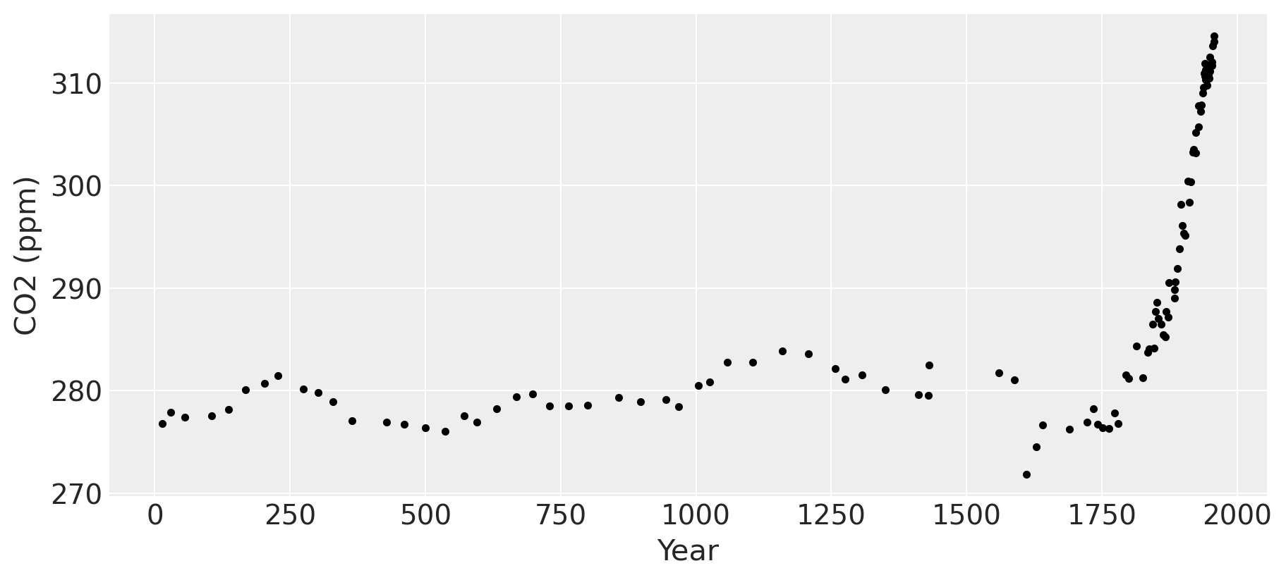
The industrial revolution era occurred around the years 1760 to 1840. This point is clearly visible in the graph, where CO2 levels rise dramatically after being fairly stationary at around 280 ppm for over a thousand years.

Uncertainty in ‘x’

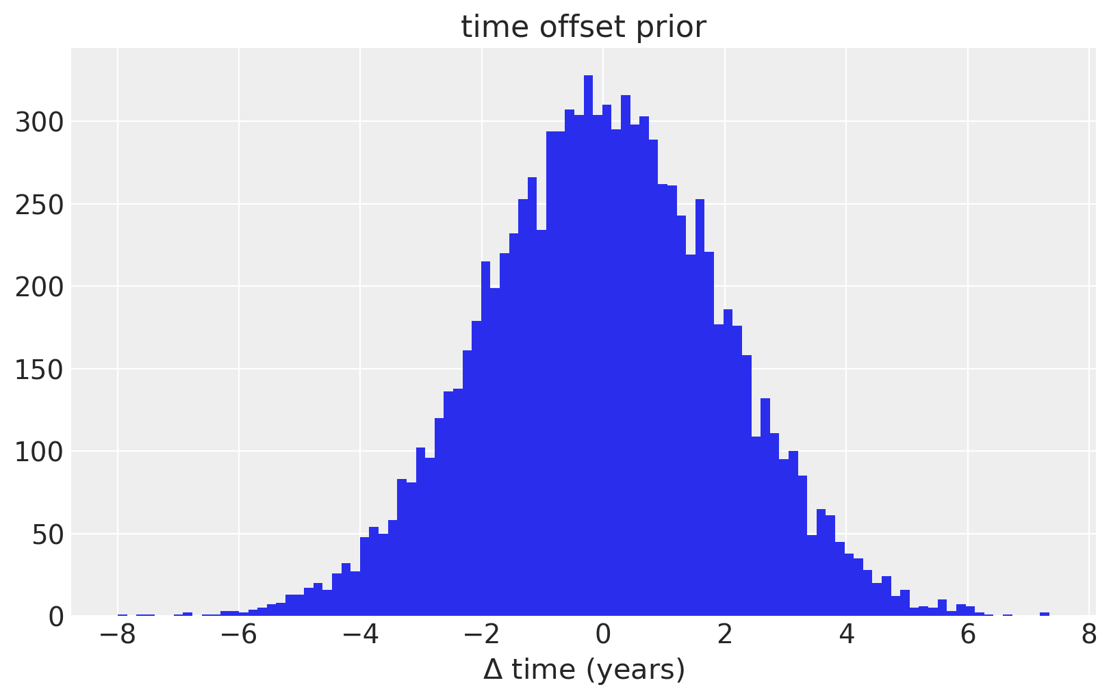
To model uncertainty in \(x\), or time, we place a prior distribution over each of the observation dates. So that the prior is standardized, we specifically use a PyMC3 random variable to model the difference between the date given in the data set, and it’s error. We assume that these differences are normal with mean zero, and standard deviation of two years. We also enforce that the observations have a strict ordering in time using the ordered transform.

For just the ice core data, the uncertainty in \(x\) is not very important. In the last example, we’ll see how it plays a more influential role in the model.

fig = plt.figure(figsize=(8, 5))
ax = plt.gca()
ax.hist(100 * pm.Normal.dist(mu=0.0, sigma=0.02).random(size=10000), 100)
ax.set_xlabel(r"$\Delta$ time (years)")
ax.set_title("time offset prior");

t = ice.year.values
y = ice.CO2.values

# normalize the CO2 readings prior to fitting the model
y_mu, y_sd = np.mean(y[0:50]), np.std(y)
y_n = (y - y_mu) / y_sd

# scale t to have units of centuries
t_n = t / 100

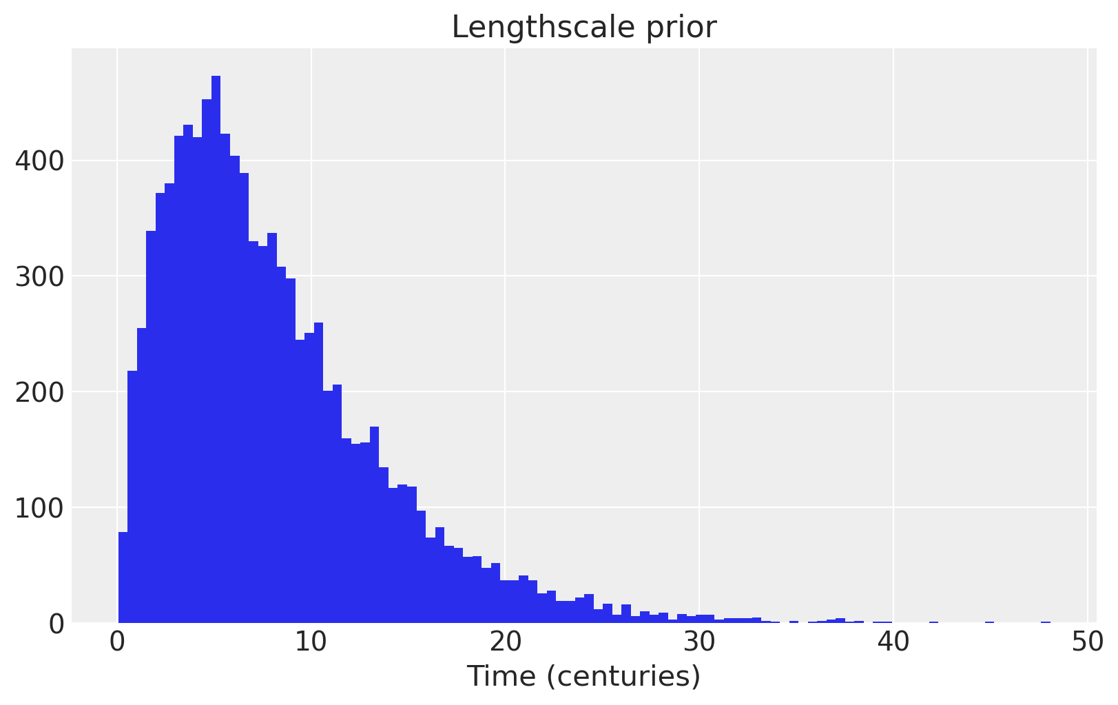
We use an informative prior on the lengthscale that places most of the mass between a few and 20 centuries.

fig = plt.figure(figsize=(8, 5))
ax = plt.gca()
ax.hist(pm.Gamma.dist(alpha=2, beta=0.25).random(size=10000), 100)
ax.set_xlabel("Time (centuries)")
ax.set_title("Lengthscale prior");

with pm.Model() as model:
    η = pm.HalfNormal("η", sigma=5)
    ℓ = pm.Gamma("ℓ", alpha=4, beta=2)
    α = pm.Gamma("α", alpha=3, beta=1)
    cov = η**2 * pm.gp.cov.RatQuad(1, α, ℓ)

    gp = pm.gp.Marginal(cov_func=cov)

    # x location uncertainty
    # - sd = 0.02 says the uncertainty on the point is about two years
    t_diff = pm.Normal("t_diff", mu=0.0, sigma=0.02, shape=len(t))
    t_uncert = t_n - t_diff

    # white noise variance
    σ = pm.HalfNormal("σ", sigma=5, testval=1)
    y_ = gp.marginal_likelihood("y", X=t_uncert[:, None], y=y_n, noise=σ)

/Users/alex_andorra/tptm_alex/pymc3/pymc3/gp/cov.py:93: UserWarning: Only 1 column(s) out of Subtensor{int64}.0 are being used to compute the covariance function. If this is not intended, increase 'input_dim' parameter to the number of columns to use. Ignore otherwise.
  " the number of columns to use. Ignore otherwise.", UserWarning)

Next we can sample with the NUTS MCMC algorithm. We run two chains but set the number of cores to one, since the linear algebra libraries used internally by Theano are multicore.

with model:
    tr = pm.sample(target_accept=0.95, return_inferencedata=True)

Auto-assigning NUTS sampler...
Initializing NUTS using jitter+adapt_diag...
Multiprocess sampling (4 chains in 4 jobs)
NUTS: [σ, t_diff, α, ℓ, η]

100.00% [8000/8000 02:07<00:00 Sampling 4 chains, 0 divergences]

Sampling 4 chains for 1_000 tune and 1_000 draw iterations (4_000 + 4_000 draws total) took 136 seconds.

az.plot_trace(tr, var_names=["t_diff"], compact=True);

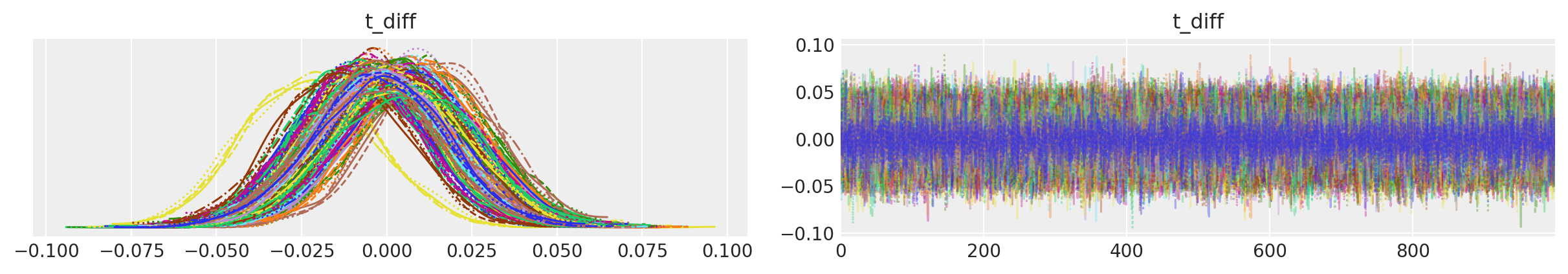
In the traceplot for t_diff, we can see that the posterior peaks for the different inputs haven’t moved much, but the uncertainty in location is accounted for by the sampling.

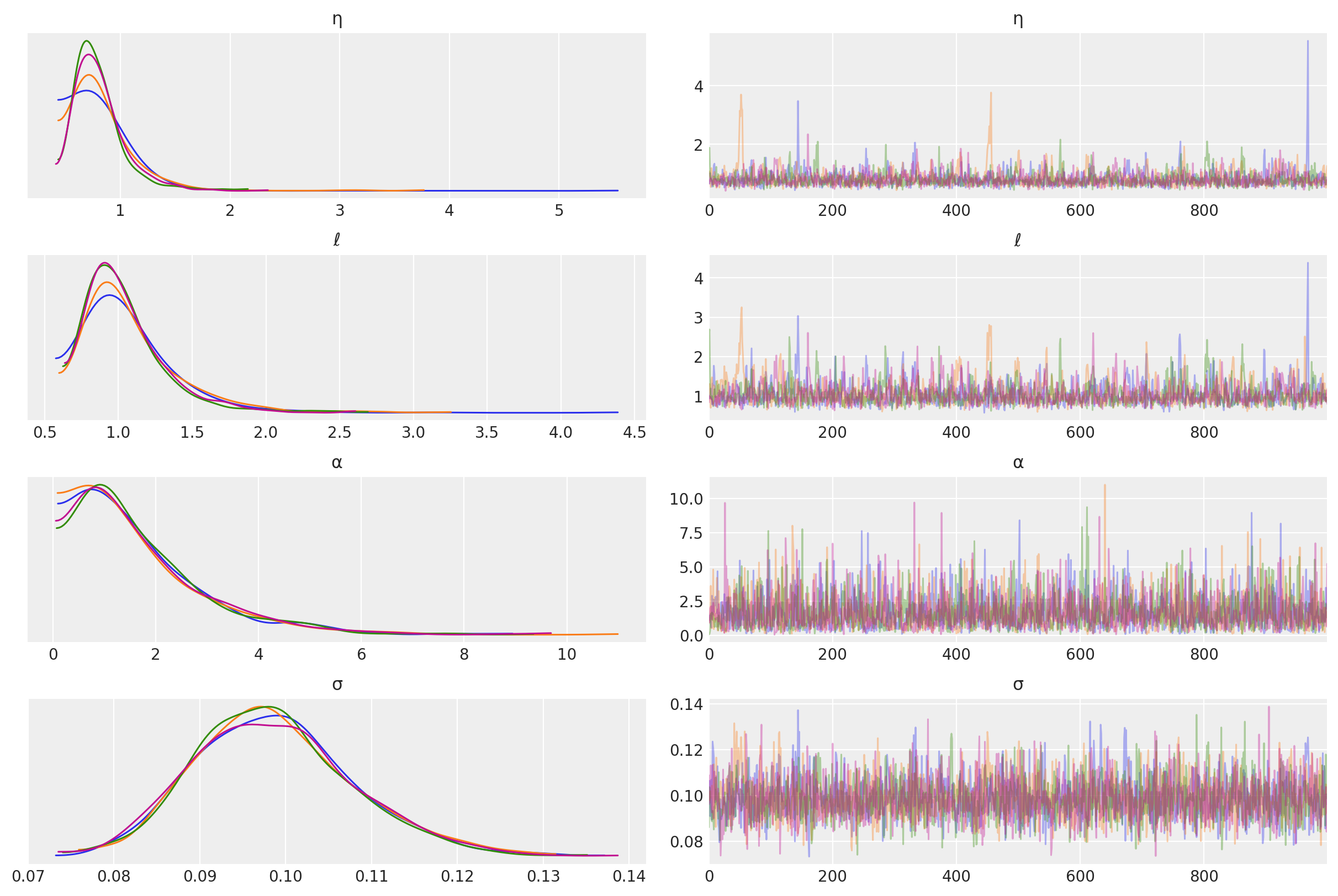
The posterior distributions for the other unknown hyperparameters is below.

az.plot_trace(tr, var_names=["η", "ℓ", "α", "σ"]);

Predictions

tnew = np.linspace(-100, 2150, 2000) * 0.01
with model:
    fnew = gp.conditional("fnew", Xnew=tnew[:, None])

with model:
    ppc = pm.sample_posterior_predictive(tr, samples=100, var_names=["fnew"])

/Users/alex_andorra/tptm_alex/pymc3/pymc3/gp/cov.py:93: UserWarning: Only 1 column(s) out of Subtensor{int64}.0 are being used to compute the covariance function. If this is not intended, increase 'input_dim' parameter to the number of columns to use. Ignore otherwise.
  " the number of columns to use. Ignore otherwise.", UserWarning)
/Users/alex_andorra/tptm_alex/pymc3/pymc3/sampling.py:1708: UserWarning: samples parameter is smaller than nchains times ndraws, some draws and/or chains may not be represented in the returned posterior predictive sample
  "samples parameter is smaller than nchains times ndraws, some draws "

100.00% [100/100 09:05<00:00]

samples = y_sd * ppc["fnew"] + y_mu

fig = plt.figure(figsize=(12, 5))
ax = plt.gca()
pm.gp.util.plot_gp_dist(ax, samples, tnew * 100, plot_samples=True, palette="Blues")
ax.plot(t, y, "k.")
ax.set_xlim([-100, 2200])
ax.set_ylabel("CO2")
ax.set_xlabel("Year");

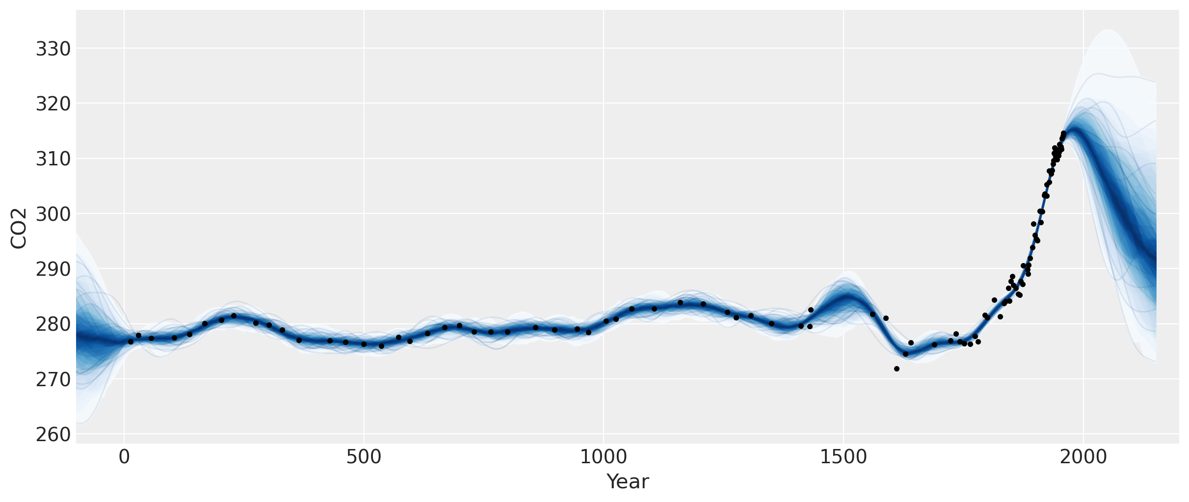
Two features are apparent in this plot. One is the little ice age, whose effects on CO2 occurs from around 1600 to 1800. The next is the industrial revolution, when people began releasing large amounts of CO2 into the atmosphere.

Semiparametric Gaussian process

The forecast past the latest data point in 1958 rises, then flattens, then dips back downwards. Should we trust this forecast? We know it hasn’t been born out (see the previous notebook) as CO2 levels have continued to rise.

We didn’t specify a mean function in our model, so we’ve assumed that our GP has a mean of zero. This means that as we forecast into the future, the function will eventually return to zero. Is this reasonable in this case? There have been no global events that suggest that atmospheric CO2 will not continue on its current trend.

A linear model for changepoints

We adopt the formulation used by Facebook’s prophet time series model. This is a linear piecewise function, where each segments endpoints are restricted to be connect to one another. Some example functions are plotted below.

def dm_changepoints(t, changepoints_t):
    A = np.zeros((len(t), len(changepoints_t)))
    for i, t_i in enumerate(changepoints_t):
        A[t >= t_i, i] = 1
    return A

For later use, we reprogram this function using symbolic theano variables. The code is a bit inscrutible, but it returns the same thing as dm_changepoitns while avoiding the use of a loop.

def dm_changepoints_theano(X, changepoints_t):
    return 0.5 * (1.0 + tt.sgn(tt.tile(X, (1, len(changepoints_t))) - changepoints_t))

From looking at the graph, some possible locations for changepoints are at 1600, 1800 and maybe 1900. These bookend the little ice age, the start of the industrial revolution, and the start of more modern industrial practices.

changepoints_t = np.array([16, 18, 19])

A = dm_changepoints(t_n, changepoints_t)

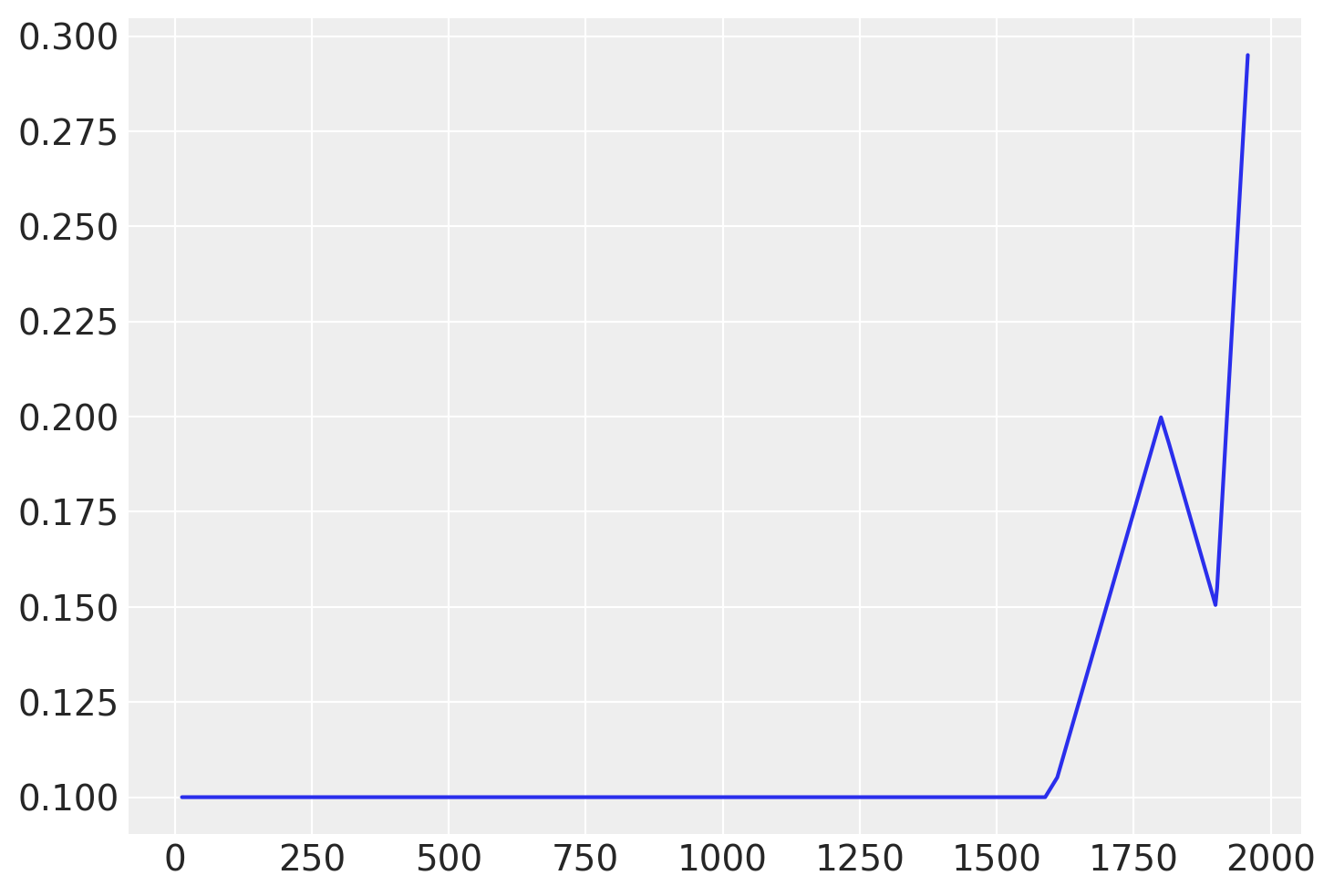
There are several parameters (which we will estimate), some test values and a plot of the resulting function is shown below

# base growth rate, or initial slope
k = 0.0

# offset
m = 0.1

# slope parameters
delta = np.array([0.05, -0.1, 0.3])

x = (k + np.dot(A, delta)) * t_n + (m + np.dot(A, -changepoints_t * delta))
plt.plot(t, x);

A custom changepoint mean function

We could encode this mean function directly, but if we wrap it inside of a Mean object, then it easier to use other Gaussian process functionality, like the .conditional and .predict methods. Look here for more information on custom mean and covariance functions. We only need to define __init__ and __call__ functions.

class PiecewiseLinear(pm.gp.mean.Mean):
    def __init__(self, changepoints, k, m, delta):
        self.changepoints = changepoints
        self.k = k
        self.m = m
        self.delta = delta

    def __call__(self, X):
        # X are the x locations, or time points
        A = dm_changepoints_theano(X, self.changepoints)
        return (self.k + tt.dot(A, self.delta)) * X.flatten() + (
            self.m + tt.dot(A, -self.changepoints * self.delta)
        )

It is inefficient to recreate A every time the mean function is evaluated, but we’ll need to do this when the number of inputs changes when making predictions.

Semiparametric changepoint model

Next is the updated model with the changepoint mean function.

with pm.Model() as model:
    η = pm.HalfNormal("η", sigma=2)
    ℓ = pm.Gamma("ℓ", alpha=4, beta=2)
    α = pm.Gamma("α", alpha=3, beta=1)
    cov = η**2 * pm.gp.cov.RatQuad(1, α, ℓ)

    # piecewise linear mean function
    k = pm.Normal("k", mu=0, sigma=1)
    m = pm.Normal("m", mu=0, sigma=1)
    delta = pm.Normal("delta", mu=0, sigma=5, shape=len(changepoints_t))
    mean = PiecewiseLinear(changepoints_t, k, m, delta)

    # include mean function in GP constructor
    gp = pm.gp.Marginal(cov_func=cov, mean_func=mean)

    # x location uncertainty
    # - sd = 0.02 says the uncertainty on the point is about two years
    t_diff = pm.Normal("t_diff", mu=0.0, sigma=0.02, shape=len(t))
    t_uncert = t_n - t_diff

    # white noise variance
    σ = pm.HalfNormal("σ", sigma=5)
    y_ = gp.marginal_likelihood("y", X=t_uncert[:, None], y=y_n, noise=σ)

/Users/alex_andorra/tptm_alex/pymc3/pymc3/gp/cov.py:93: UserWarning: Only 1 column(s) out of Subtensor{int64}.0 are being used to compute the covariance function. If this is not intended, increase 'input_dim' parameter to the number of columns to use. Ignore otherwise.
  " the number of columns to use. Ignore otherwise.", UserWarning)

with model:
    tr = pm.sample(chains=2, target_accept=0.95)

Auto-assigning NUTS sampler...
Initializing NUTS using jitter+adapt_diag...
Multiprocess sampling (2 chains in 4 jobs)
NUTS: [σ, t_diff, delta, m, k, α, ℓ, η]

100.00% [4000/4000 03:22<00:00 Sampling 2 chains, 0 divergences]

Sampling 2 chains for 1_000 tune and 1_000 draw iterations (2_000 + 2_000 draws total) took 208 seconds.

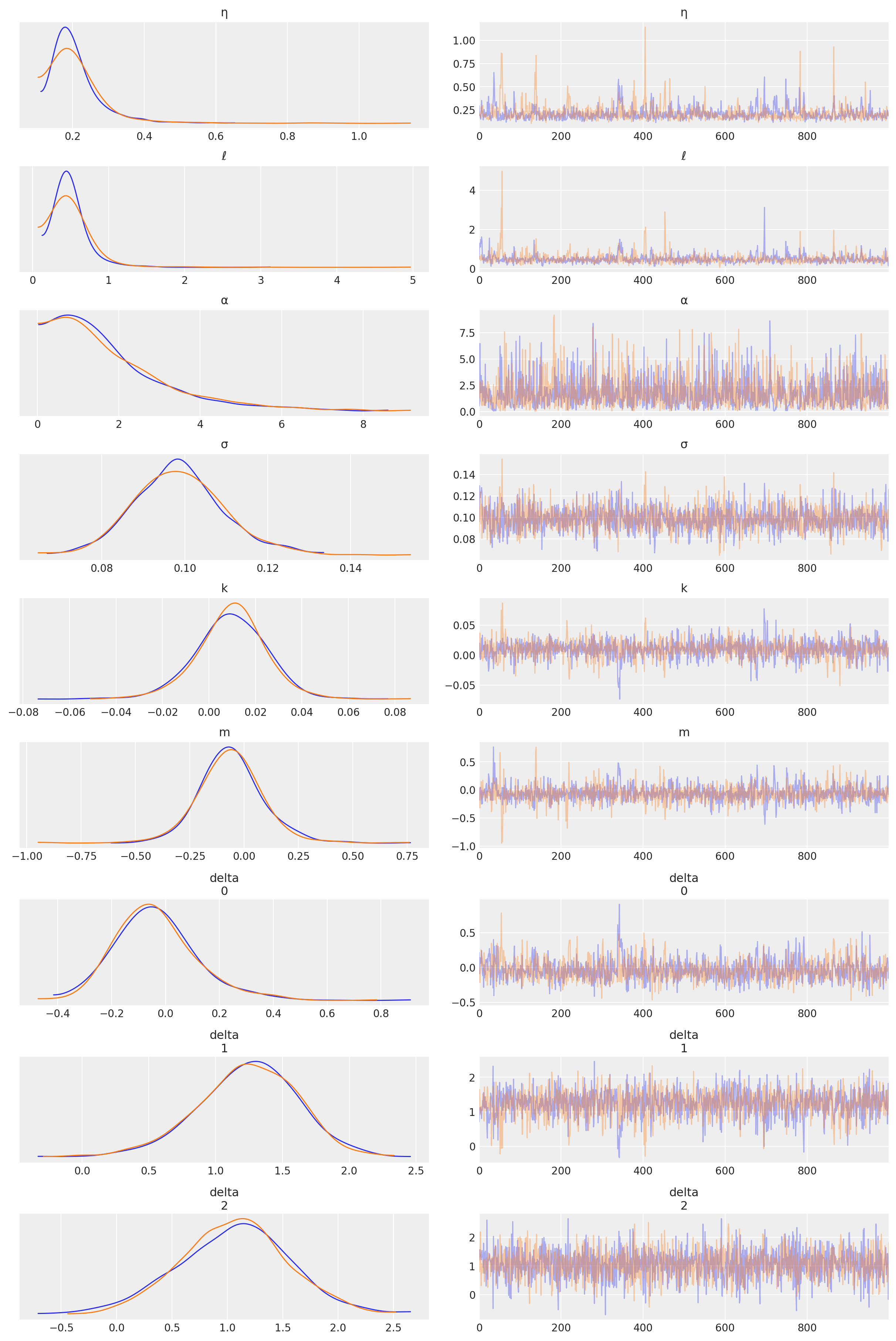
az.plot_trace(tr, var_names=["η", "ℓ", "α", "σ", "k", "m", "delta"]);

/Users/alex_andorra/opt/anaconda3/envs/dev-pymc/lib/python3.6/site-packages/arviz/data/io_pymc3.py:89: FutureWarning: Using `from_pymc3` without the model will be deprecated in a future release. Not using the model will return less accurate and less useful results. Make sure you use the model argument or call from_pymc3 within a model context.
  FutureWarning,

Predictions

tnew = np.linspace(-100, 2200, 2000) * 0.01

with model:
    fnew = gp.conditional("fnew", Xnew=tnew[:, None])

with model:
    ppc = pm.sample_posterior_predictive(tr, samples=100, var_names=["fnew"])

/Users/alex_andorra/tptm_alex/pymc3/pymc3/gp/cov.py:93: UserWarning: Only 1 column(s) out of Subtensor{int64}.0 are being used to compute the covariance function. If this is not intended, increase 'input_dim' parameter to the number of columns to use. Ignore otherwise.
  " the number of columns to use. Ignore otherwise.", UserWarning)
/Users/alex_andorra/tptm_alex/pymc3/pymc3/sampling.py:1708: UserWarning: samples parameter is smaller than nchains times ndraws, some draws and/or chains may not be represented in the returned posterior predictive sample
  "samples parameter is smaller than nchains times ndraws, some draws "

100.00% [100/100 04:27<00:00]

samples = y_sd * ppc["fnew"] + y_mu

fig = plt.figure(figsize=(12, 5))
ax = plt.gca()
pm.gp.util.plot_gp_dist(ax, samples, tnew * 100, plot_samples=True, palette="Blues")
ax.plot(t, y, "k.")
ax.set_xlim([-100, 2200])
ax.set_ylabel("CO2 (ppm)")
ax.set_xlabel("year");

These results look better, but we had to choose exactly where the changepoints were. Instead of using a changepoint in the mean function, we could also specify this same changepoint behavior in the form of a covariance function. One benefit of the latter formulation is that the changepoint can be a more realistic smooth transition, instead of a discrete breakpoint. In the next section, we’ll look at how to do this.

A custom changepoint covariance function

More complex covariance functions can be constructed by composing base covariance functions in several ways. For instance, two of the most commonly used operations are

• The sum of two covariance functions is a covariance function

• The product of two covariance functions is a covariance function

We can also construct a covariance function by scaling a base covariance function (\(k_b\)) by any arbitrary function, $\( k(x, x) = s(x) k_{\mathrm{b}}(x, x') s(x') \,. \)$ The scaling function can be parameterized by known parameters, or unknown parameters can be inferred.

Heaviside step function

To specifically construct a covariance function that describes a changepoint, we could propose a scaling function \(s(x)\) that specifies the region where the base covariance is active. The simplest option is the step function,

\[\begin{split} s(x;\, x_0) = \begin{cases} 0 & x \leq x_0 \\ 1 & x_0 < x \end{cases} \end{split}\]

which is parameterized by the changepoint \(x_0\). The covariance function \(s(x; x_0) k_b(x, x') s(x'; x_0)\) is only active in the region \(x > x_0\).

The PyMC3 contains the ScaledCov covariance function. As arguments, it takes a base covariance, a scaling function, and the tuple of the arguments for the base covariance. To construct this in PyMC3, we first define the scaling function:

def step_function(x, x0, greater=True):
    if greater:
        # s = 1 for x > x_0
        return 0.5 * (tt.sgn(x - x0) + 1.0)
    else:
        return 0.5 * (tt.sgn(x0 - x) + 1.0)

step_function(np.linspace(0, 10, 10), x0=5, greater=True).eval()

array([0., 0., 0., 0., 0., 1., 1., 1., 1., 1.])

step_function(np.linspace(0, 10, 10), x0=5, greater=False).eval()

array([1., 1., 1., 1., 1., 0., 0., 0., 0., 0.])

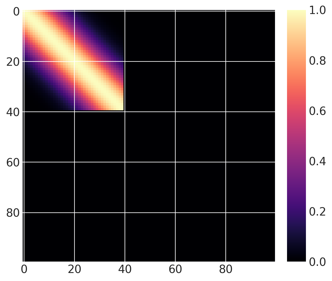
Then we can define the the following covariance function, that we compute over \(x \in (0, 100)\). The base covariance has a lengthscale of 10, and \(x_0 = 40\). Since we are using a step function, it is “active” for \(x \leq 40\) when greater=False, and for for \(x > 40\) when greater=True.

cov = pm.gp.cov.ExpQuad(1, 10)
sc_cov = pm.gp.cov.ScaledCov(1, cov, step_function, (40, False))

x = np.linspace(0, 100, 100)
K = sc_cov(x[:, None]).eval()
m = plt.imshow(K, cmap="magma")
plt.colorbar(m);

/Users/alex_andorra/tptm_alex/pymc3/pymc3/gp/cov.py:93: UserWarning: Only 1 column(s) out of Subtensor{int64}.0 are being used to compute the covariance function. If this is not intended, increase 'input_dim' parameter to the number of columns to use. Ignore otherwise.
  " the number of columns to use. Ignore otherwise.", UserWarning)

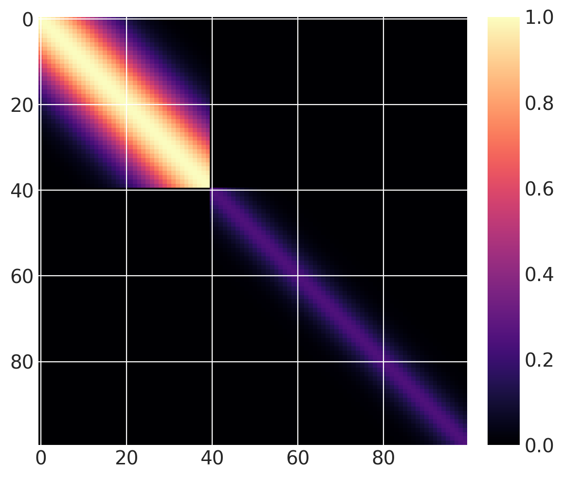
But this isn’t a changepoint covariance function yet. We can add two of these together. For \(x > 40\), let’s use a base covariance that is a Matern32 with a lengthscale of 5 and an amplitude of 0.25:

cov1 = pm.gp.cov.ExpQuad(1, 10)
sc_cov1 = pm.gp.cov.ScaledCov(1, cov1, step_function, (40, False))

cov2 = 0.25 * pm.gp.cov.Matern32(1, 5)
sc_cov2 = pm.gp.cov.ScaledCov(1, cov2, step_function, (40, True))

sc_cov = sc_cov1 + sc_cov2

# plot over 0 < x < 100
x = np.linspace(0, 100, 100)
K = sc_cov(x[:, None]).eval()
m = plt.imshow(K, cmap="magma")
plt.colorbar(m);

/Users/alex_andorra/tptm_alex/pymc3/pymc3/gp/cov.py:93: UserWarning: Only 1 column(s) out of Subtensor{int64}.0 are being used to compute the covariance function. If this is not intended, increase 'input_dim' parameter to the number of columns to use. Ignore otherwise.
  " the number of columns to use. Ignore otherwise.", UserWarning)
/Users/alex_andorra/tptm_alex/pymc3/pymc3/gp/cov.py:93: UserWarning: Only 1 column(s) out of Subtensor{int64}.0 are being used to compute the covariance function. If this is not intended, increase 'input_dim' parameter to the number of columns to use. Ignore otherwise.
  " the number of columns to use. Ignore otherwise.", UserWarning)

What do samples from the Gaussian process prior with this covariance look like?

prior_samples = np.random.multivariate_normal(np.zeros(100), K, 3).T
plt.plot(x, prior_samples)
plt.axvline(x=40, color="k", alpha=0.5);

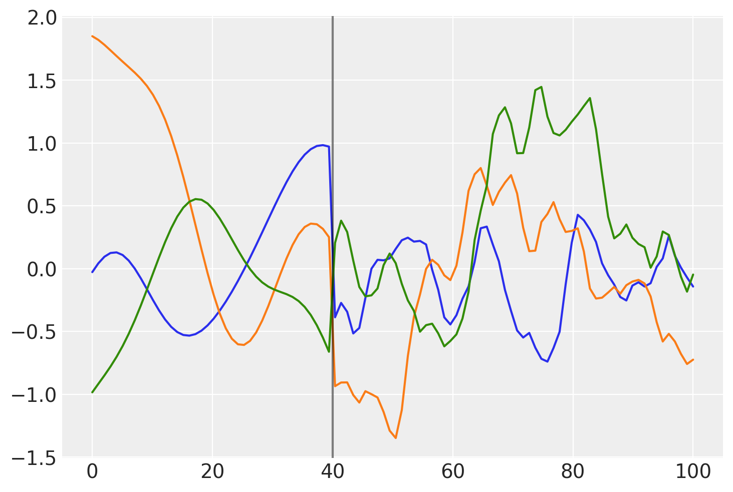
Before \(x = 40\), the function is smooth and slowly changing. After \(x = 40\), the samples are less smooth and change quickly.

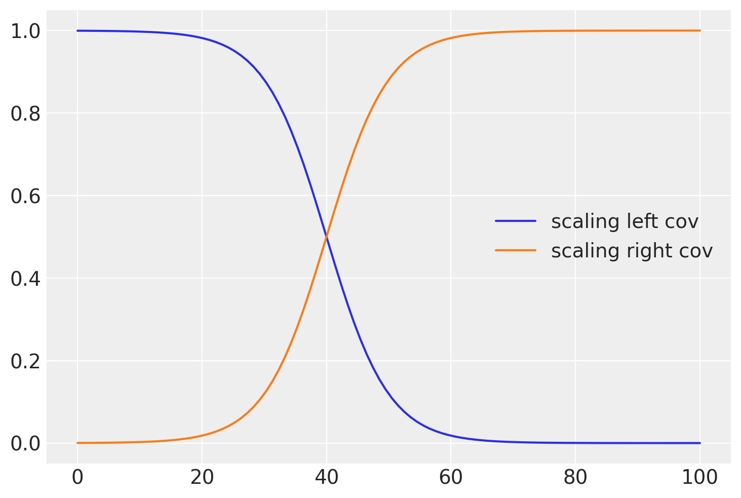
A gradual change with a sigmoid function

Instead of a sharp cutoff, It is usually more realistic to have a smooth transition. For this we can use the logistic function, shown below:

# b is the slope, a is the location

b = -0.2
a = 40
plt.plot(x, pm.math.invlogit(b * (x - a)).eval(), label="scaling left cov")

b = 0.2
a = 40
plt.plot(x, pm.math.invlogit(b * (x - a)).eval(), label="scaling right cov")
plt.legend();

def logistic(x, b, x0):
    # b is the slope, x0 is the location
    return pm.math.invlogit(b * (x - x0))

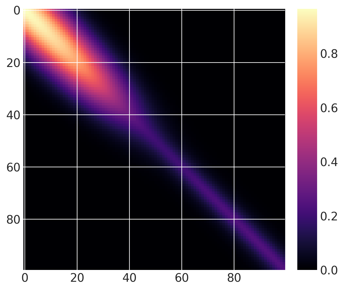
The same covariance function as before, but with a gradual changepoint is shown below:

cov1 = pm.gp.cov.ExpQuad(1, 10)
sc_cov1 = pm.gp.cov.ScaledCov(1, cov1, logistic, (-0.1, 40))

cov2 = 0.25 * pm.gp.cov.Matern32(1, 5)
sc_cov2 = pm.gp.cov.ScaledCov(1, cov2, logistic, (0.1, 40))

sc_cov = sc_cov1 + sc_cov2

# plot over 0 < x < 100
x = np.linspace(0, 100, 100)
K = sc_cov(x[:, None]).eval()
m = plt.imshow(K, cmap="magma")
plt.colorbar(m);

/Users/alex_andorra/tptm_alex/pymc3/pymc3/gp/cov.py:93: UserWarning: Only 1 column(s) out of Subtensor{int64}.0 are being used to compute the covariance function. If this is not intended, increase 'input_dim' parameter to the number of columns to use. Ignore otherwise.
  " the number of columns to use. Ignore otherwise.", UserWarning)

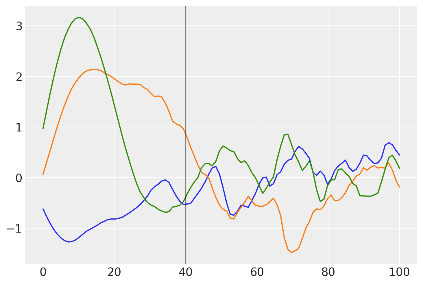
Below, you can see that the transition of the prior functions from one region to the next is more gradual:

prior_samples = np.random.multivariate_normal(np.zeros(100), K, 3).T
plt.plot(x, prior_samples)
plt.axvline(x=40, color="k", alpha=0.5);

Lets try this model out instead of the semiparametric changepoint version.

Changepoint covariance model

The features of this model are:

• One covariance for short term variation across all time points

• The parameter x0 is the location of the industrial revolution. It is given a prior that has most of its support between years 1760 and 1840, centered at 1800.

• We can easily use this x0 parameter as the shift parameter in the 2nd degree Polynomial (quadratic) covariance, and as the location of the changepoint in the changepoint covariance.

• A changepoint covariance that is ExpQuad prior to the industrial revolution, and ExpQuad + Polynomial(degree=2) afterwards.

• We use the same scaling and lengthscale parameters for each of the two base covariances in the changepoint covariance.

• Still modeling uncertainty in x as before.

with pm.Model() as model:
    η = pm.HalfNormal("η", sigma=5)
    ℓ = pm.Gamma("ℓ", alpha=2, beta=0.1)

    # changepoint occurs near the year 1800, sometime between 1760, 1840
    x0 = pm.Normal("x0", mu=18, sigma=0.1)
    # the change happens gradually
    a = pm.HalfNormal("a", sigma=2)
    # a constant for the
    c = pm.HalfNormal("c", sigma=3)
    # quadratic polynomial scale
    ηq = pm.HalfNormal("ηq", sigma=5)

    cov1 = η**2 * pm.gp.cov.ExpQuad(1, ℓ)
    cov2 = η**2 * pm.gp.cov.ExpQuad(1, ℓ) + ηq**2 * pm.gp.cov.Polynomial(1, x0, 2, c)

    # construct changepoint cov
    sc_cov1 = pm.gp.cov.ScaledCov(1, cov1, logistic, (-a, x0))
    sc_cov2 = pm.gp.cov.ScaledCov(1, cov2, logistic, (a, x0))
    cov_c = sc_cov1 + sc_cov2

    # short term variation
    ηs = pm.HalfNormal("ηs", sigma=5)
    ℓs = pm.Gamma("ℓs", alpha=2, beta=1)
    cov_s = ηs**2 * pm.gp.cov.Matern52(1, ℓs)

    gp = pm.gp.Marginal(cov_func=cov_s + cov_c)

    t_diff = pm.Normal("t_diff", mu=0.0, sigma=0.02, shape=len(t))
    t_uncert = t_n - t_diff

    # white noise variance
    σ = pm.HalfNormal("σ", sigma=5, testval=1)
    y_ = gp.marginal_likelihood("y", X=t_uncert[:, None], y=y_n, noise=σ)

/Users/alex_andorra/tptm_alex/pymc3/pymc3/gp/cov.py:93: UserWarning: Only 1 column(s) out of Subtensor{int64}.0 are being used to compute the covariance function. If this is not intended, increase 'input_dim' parameter to the number of columns to use. Ignore otherwise.
  " the number of columns to use. Ignore otherwise.", UserWarning)
/Users/alex_andorra/tptm_alex/pymc3/pymc3/gp/cov.py:93: UserWarning: Only 1 column(s) out of Subtensor{int64}.0 are being used to compute the covariance function. If this is not intended, increase 'input_dim' parameter to the number of columns to use. Ignore otherwise.
  " the number of columns to use. Ignore otherwise.", UserWarning)
/Users/alex_andorra/tptm_alex/pymc3/pymc3/gp/cov.py:93: UserWarning: Only 1 column(s) out of Subtensor{int64}.0 are being used to compute the covariance function. If this is not intended, increase 'input_dim' parameter to the number of columns to use. Ignore otherwise.
  " the number of columns to use. Ignore otherwise.", UserWarning)

with model:
    tr = pm.sample(500, chains=2, target_accept=0.95)

Auto-assigning NUTS sampler...
Initializing NUTS using jitter+adapt_diag...
Multiprocess sampling (2 chains in 4 jobs)
NUTS: [σ, t_diff, ℓs, ηs, ηq, c, a, x0, ℓ, η]

100.00% [3000/3000 02:27<00:00 Sampling 2 chains, 0 divergences]

Sampling 2 chains for 1_000 tune and 500 draw iterations (2_000 + 1_000 draws total) took 151 seconds.

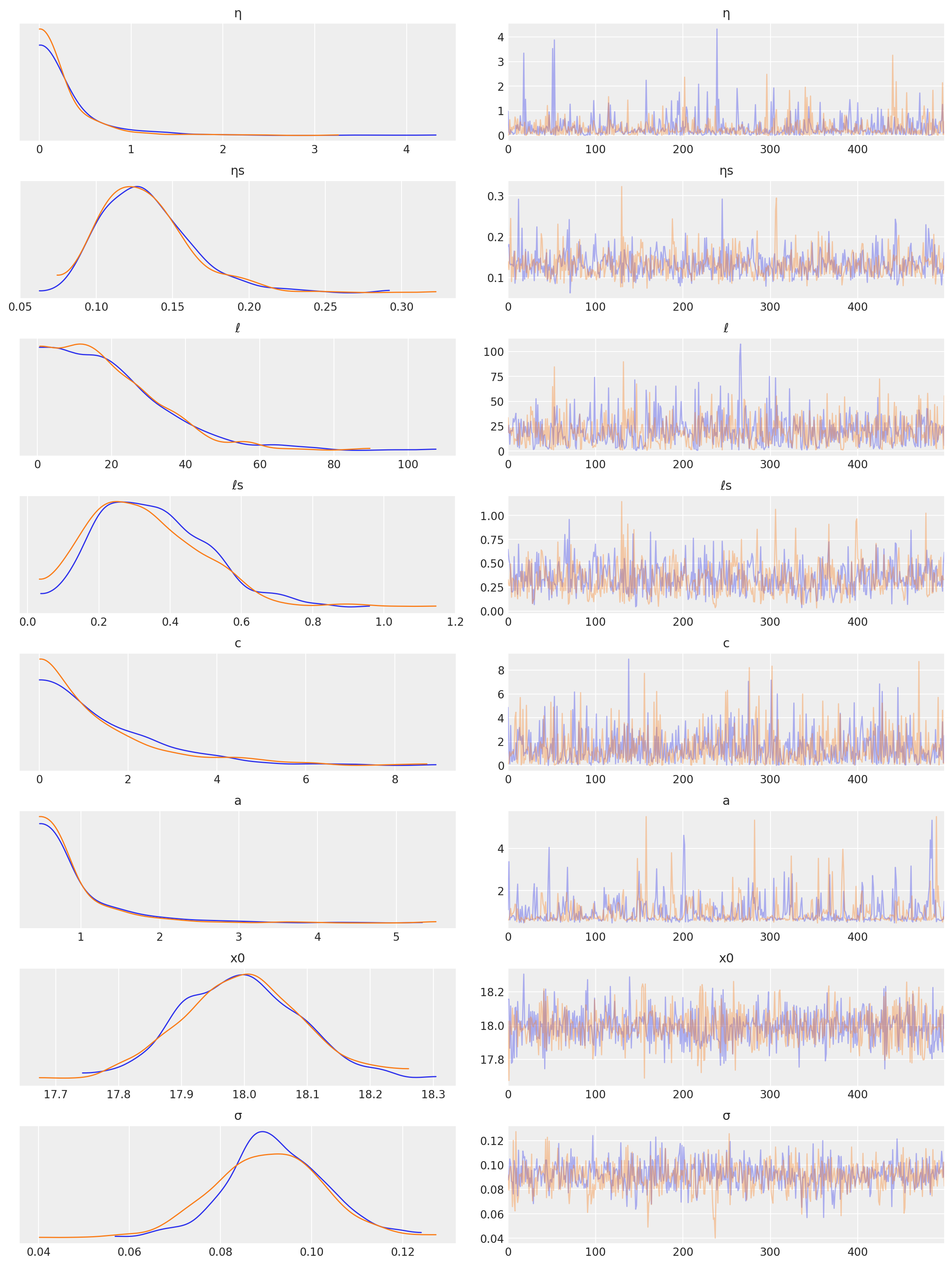
az.plot_trace(tr, var_names=["η", "ηs", "ℓ", "ℓs", "c", "a", "x0", "σ"]);

/Users/alex_andorra/opt/anaconda3/envs/dev-pymc/lib/python3.6/site-packages/arviz/data/io_pymc3.py:89: FutureWarning: Using `from_pymc3` without the model will be deprecated in a future release. Not using the model will return less accurate and less useful results. Make sure you use the model argument or call from_pymc3 within a model context.
  FutureWarning,

Predictions

tnew = np.linspace(-100, 2300, 2200) * 0.01

with model:
    fnew = gp.conditional("fnew", Xnew=tnew[:, None])

with model:
    ppc = pm.sample_posterior_predictive(tr, samples=100, var_names=["fnew"])

/Users/alex_andorra/tptm_alex/pymc3/pymc3/gp/cov.py:93: UserWarning: Only 1 column(s) out of Subtensor{int64}.0 are being used to compute the covariance function. If this is not intended, increase 'input_dim' parameter to the number of columns to use. Ignore otherwise.
  " the number of columns to use. Ignore otherwise.", UserWarning)
/Users/alex_andorra/tptm_alex/pymc3/pymc3/sampling.py:1708: UserWarning: samples parameter is smaller than nchains times ndraws, some draws and/or chains may not be represented in the returned posterior predictive sample
  "samples parameter is smaller than nchains times ndraws, some draws "

100.00% [100/100 06:35<00:00]

samples = y_sd * ppc["fnew"] + y_mu

fig = plt.figure(figsize=(12, 5))
ax = plt.gca()
pm.gp.util.plot_gp_dist(ax, samples, tnew, plot_samples=True, palette="Blues")
ax.plot(t / 100, y, "k.")
ax.set_xticks(np.arange(0, 23))
ax.set_xlim([-1, 23])
ax.set_ylim([250, 450])
ax.set_xlabel("time (in centuries)")
ax.set_ylabel("CO2 (ppm)");

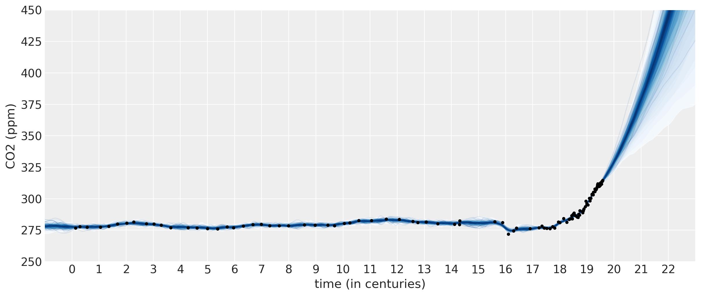
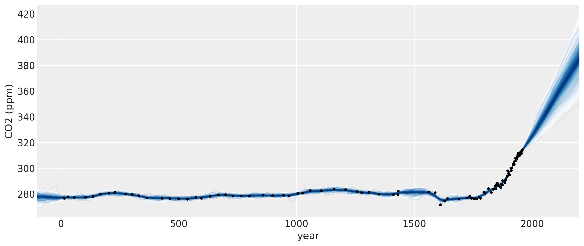
The predictions for this model look much more realistic. The sum of a 2nd degree polynomial with an ExpQuad looks like a good model to forecast with. It allows for the amount of CO2 to increase in a not-exactly-linear fashion. We can see from the predictions that:

• The amount of CO2 could increase at a faster rate

• The amount of CO2 should increase more or less linearly

• It is possible for the CO2 to start to decrease

Incorporating Atmospheric CO2 measurements

Next, we incorporate the CO2 measurements from the Mauna Loa observatory. These data points were taken monthly from atmospheric levels. Unlike the ice core data, there is no uncertainty in these measurements. While modeling both of these data sets together, the value of including the uncertainty in the ice core measurement time will be more apparent. Hintcasting the Mauna Loa seasonality using ice core data doesn’t make too much sense, since the seasonality pattern at the south pole is different than that in the northern hemisphere in Hawaii. We’ll show it anyways though since it’s possible, and may be useful in other contexts.

First let’s load in the data, and then plot it alongside the ice core data.

import time

from datetime import datetime as dt


def toYearFraction(date):
    date = pd.to_datetime(date)

    def sinceEpoch(date):  # returns seconds since epoch
        return time.mktime(date.timetuple())

    s = sinceEpoch

    year = date.year
    startOfThisYear = dt(year=year, month=1, day=1)
    startOfNextYear = dt(year=year + 1, month=1, day=1)

    yearElapsed = s(date) - s(startOfThisYear)
    yearDuration = s(startOfNextYear) - s(startOfThisYear)
    fraction = yearElapsed / yearDuration

    return date.year + fraction

airdata = pd.read_csv(pm.get_data("monthly_in_situ_co2_mlo.csv"), header=56)

# - replace -99.99 with NaN
airdata.replace(to_replace=-99.99, value=np.nan, inplace=True)

# fix column names
cols = [
    "year",
    "month",
    "--",
    "--",
    "CO2",
    "seasonaly_adjusted",
    "fit",
    "seasonally_adjusted_fit",
    "CO2_filled",
    "seasonally_adjusted_filled",
]
airdata.columns = cols
cols.remove("--")
cols.remove("--")
airdata = airdata[cols]

# drop rows with nan
airdata.dropna(inplace=True)

# fix time index
airdata["day"] = 15
airdata.index = pd.to_datetime(airdata[["year", "month", "day"]])
airdata["year"] = [toYearFraction(date) for date in airdata.index.values]
cols.remove("month")
airdata = airdata[cols]

air = airdata[["year", "CO2"]]
air.head(5)

	year	CO2
1958-03-15	1958.200000	315.69
1958-04-15	1958.284932	317.46
1958-05-15	1958.367123	317.50
1958-07-15	1958.534247	315.86
1958-08-15	1958.619178	314.93

Like was done in the first notebook, we reserve the data from 2004 onwards as the test set.

sep_idx = air.index.searchsorted(pd.to_datetime("2003-12-15"))
air_test = air.iloc[sep_idx:, :]
air = air.iloc[: sep_idx + 1, :]

plt.plot(air.year.values, air.CO2.values, ".b", label="atmospheric CO2")
plt.plot(ice.year.values, ice.CO2.values, ".", color="c", label="ice core CO2")
plt.legend()
plt.xlabel("year")
plt.ylabel("CO2 (ppm)");

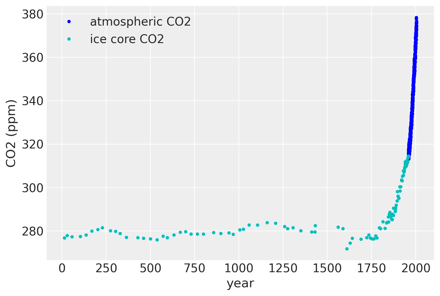
If we zoom in on the late 1950’s, we can see that the atmospheric data has a seasonal component, while the ice core data does not.

plt.plot(air.year.values, air.CO2.values, ".b", label="atmospheric CO2")
plt.plot(ice.year.values, ice.CO2.values, ".", color="c", label="ice core CO2")
plt.xlim([1949, 1965])
plt.ylim([305, 325])
plt.legend()
plt.xlabel("year")
plt.ylabel("CO2 (ppm)");

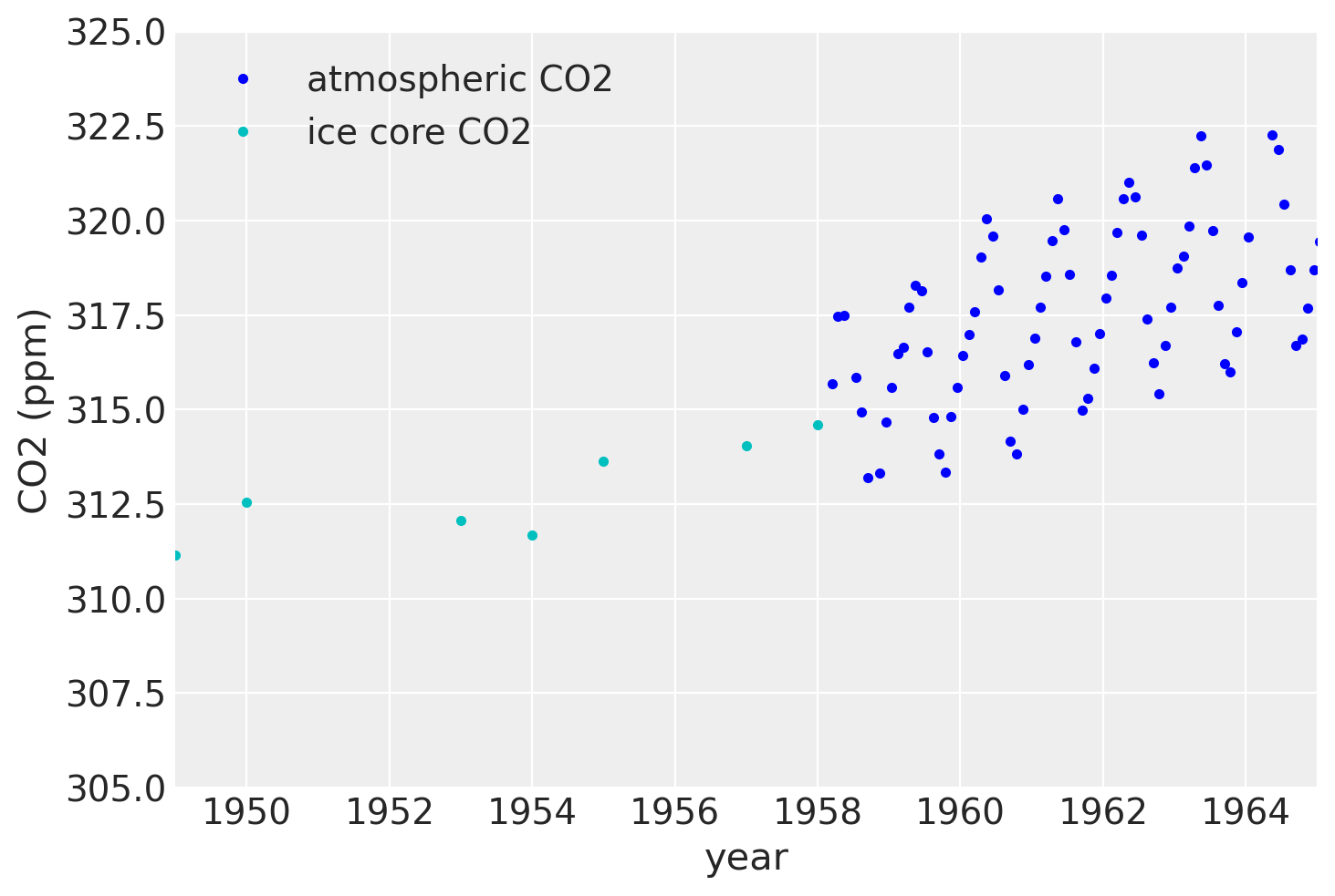
Since the ice core data isn’t measured accurately, it won’t be possible to backcast the seasonal component unless we model uncertainty in x.

To model both the data together, we will combine the model we’ve built up using the ice core data, and combine it with elements from the previous notebook on the Mauna Loa data. From the previous notebook we will additionally include the:

• The Periodic, seasonal component

• The RatQuad covariance for short range, annual scale variations

Also, since we are using two different data sets, there should be two different y-direction uncertainties, one for the ice core data, and one for the atmospheric data. To accomplish this, we make a custom WhiteNoise covariance function that has two σ parameters.

All custom covariance functions need to have the same three methods defined, __init__, diag, and full. full returns the full covariance, given either X or X and a different Xs. diag returns only the diagonal, and __init__ saves the input parameters.

class CustomWhiteNoise(pm.gp.cov.Covariance):
    """Custom White Noise covariance
    - sigma1 is applied to the first n1 points in the data
    - sigma2 is applied to the next n2 points in the data

    The total number of data points n = n1 + n2
    """

    def __init__(self, sigma1, sigma2, n1, n2):
        super().__init__(1, None)
        self.sigma1 = sigma1
        self.sigma2 = sigma2
        self.n1 = n1
        self.n2 = n2

    def diag(self, X):
        d1 = tt.alloc(tt.square(self.sigma1), self.n1)
        d2 = tt.alloc(tt.square(self.sigma2), self.n2)
        return tt.concatenate((d1, d2), 0)

    def full(self, X, Xs=None):
        if Xs is None:
            return tt.diag(self.diag(X))
        else:
            return tt.alloc(0.0, X.shape[0], Xs.shape[0])

Next we need to organize and combine the two data sets. Remember that the unit on the x-axis is centuries, not years.

# form dataset, stack t and co2 measurements
t = np.concatenate((ice.year.values, air.year.values), 0)
y = np.concatenate((ice.CO2.values, air.CO2.values), 0)

y_mu, y_sd = np.mean(ice.CO2.values[0:50]), np.std(y)
y_n = (y - y_mu) / y_sd
t_n = t * 0.01

The specification of the model is below. The dataset is larger now, so MCMC will take much longer now. But you will see that estimating the whole posterior is clearly worth the wait!

We also choose our priors for the hyperparameters more carefully. For the changepoint covariance, we model the post-industrial revolution data with an ExpQuad covariance that has the same longer lengthscale as before the industrial revolution. The idea is that whatever process was at work before, is still there after. But then we add the product of a Polynomial(degree=2) and a Matern52. We fix the lengthscale of the Matern52 to two. Since it has only been about two centuries since the industrial revolution, we force the Polynomial component to decay at that time scale. This forces the uncertainty to rise at this time scale.

The 2nd degree polynomial and Matern52 product expresses our prior belief that the CO2 levels may increase semi-quadratically, or decrease semi-quadratically, since the scaling parameter for this may also end up being zero.

with pm.Model() as model:
    ηc = pm.Gamma("ηc", alpha=3, beta=2)
    ℓc = pm.Gamma("ℓc", alpha=10, beta=1)

    # changepoint occurs near the year 1800, sometime between 1760, 1840
    x0 = pm.Normal("x0", mu=18, sigma=0.1)
    # the change happens gradually
    a = pm.Gamma("a", alpha=3, beta=1)
    # constant offset
    c = pm.HalfNormal("c", sigma=2)

    # quadratic polynomial scale
    ηq = pm.HalfNormal("ηq", sigma=1)
    ℓq = 2.0  # 2 century impact, since we only have 2 C of post IR data

    cov1 = ηc**2 * pm.gp.cov.ExpQuad(1, ℓc)
    cov2 = ηc**2 * pm.gp.cov.ExpQuad(1, ℓc) + ηq**2 * pm.gp.cov.Polynomial(
        1, x0, 2, c
    ) * pm.gp.cov.Matern52(
        1, ℓq
    )  # ~2 century impact

    # construct changepoint cov
    sc_cov1 = pm.gp.cov.ScaledCov(1, cov1, logistic, (-a, x0))
    sc_cov2 = pm.gp.cov.ScaledCov(1, cov2, logistic, (a, x0))
    gp_c = pm.gp.Marginal(cov_func=sc_cov1 + sc_cov2)

    # short term variation
    ηs = pm.HalfNormal("ηs", sigma=3)
    ℓs = pm.Gamma("ℓs", alpha=5, beta=100)
    α = pm.Gamma("α", alpha=4, beta=1)
    cov_s = ηs**2 * pm.gp.cov.RatQuad(1, α, ℓs)
    gp_s = pm.gp.Marginal(cov_func=cov_s)

    # medium term variation
    ηm = pm.HalfNormal("ηm", sigma=5)
    ℓm = pm.Gamma("ℓm", alpha=2, beta=3)
    cov_m = ηm**2 * pm.gp.cov.ExpQuad(1, ℓm)
    gp_m = pm.gp.Marginal(cov_func=cov_m)

    ## periodic
    ηp = pm.HalfNormal("ηp", sigma=2)
    ℓp_decay = pm.Gamma("ℓp_decay", alpha=40, beta=0.1)
    ℓp_smooth = pm.Normal("ℓp_smooth ", mu=1.0, sigma=0.05)
    period = 1 * 0.01  # we know the period is annual
    cov_p = ηp**2 * pm.gp.cov.Periodic(1, period, ℓp_smooth) * pm.gp.cov.ExpQuad(1, ℓp_decay)
    gp_p = pm.gp.Marginal(cov_func=cov_p)

    gp = gp_c + gp_m + gp_s + gp_p

    # - x location uncertainty (sd = 0.01 is a standard deviation of one year)
    # - only the first 111 points are the ice core data
    t_mu = t_n[:111]
    t_diff = pm.Normal("t_diff", mu=0.0, sigma=0.02, shape=len(t_mu))
    t_uncert = t_mu - t_diff
    t_combined = tt.concatenate((t_uncert, t_n[111:]), 0)

    # Noise covariance, using boundary avoiding priors for MAP estimation
    σ1 = pm.Gamma("σ1", alpha=3, beta=50)
    σ2 = pm.Gamma("σ2", alpha=3, beta=50)
    η_noise = pm.HalfNormal("η_noise", sigma=1)
    ℓ_noise = pm.Gamma("ℓ_noise", alpha=2, beta=200)
    cov_noise = η_noise**2 * pm.gp.cov.Matern32(1, ℓ_noise) + CustomWhiteNoise(σ1, σ2, 111, 545)

    y_ = gp.marginal_likelihood("y", X=t_combined[:, None], y=y_n, noise=cov_noise)

/Users/alex_andorra/tptm_alex/pymc3/pymc3/gp/cov.py:93: UserWarning: Only 1 column(s) out of Subtensor{int64}.0 are being used to compute the covariance function. If this is not intended, increase 'input_dim' parameter to the number of columns to use. Ignore otherwise.
  " the number of columns to use. Ignore otherwise.", UserWarning)
/Users/alex_andorra/tptm_alex/pymc3/pymc3/gp/cov.py:93: UserWarning: Only 1 column(s) out of Subtensor{int64}.0 are being used to compute the covariance function. If this is not intended, increase 'input_dim' parameter to the number of columns to use. Ignore otherwise.
  " the number of columns to use. Ignore otherwise.", UserWarning)
/Users/alex_andorra/tptm_alex/pymc3/pymc3/gp/cov.py:93: UserWarning: Only 1 column(s) out of Subtensor{int64}.0 are being used to compute the covariance function. If this is not intended, increase 'input_dim' parameter to the number of columns to use. Ignore otherwise.
  " the number of columns to use. Ignore otherwise.", UserWarning)

with model:
    tr = pm.sample(500, tune=1000, chains=2, cores=16, return_inferencedata=True)

Auto-assigning NUTS sampler...
Initializing NUTS using jitter+adapt_diag...
Multiprocess sampling (2 chains in 16 jobs)
NUTS: [ℓ_noise, η_noise, σ2, σ1, t_diff, ℓp_smooth , ℓp_decay, ηp, ℓm, ηm, α, ℓs, ηs, ηq, c, a, x0, ℓc, ηc]

100.00% [3000/3000 21:58:11<00:00 Sampling 2 chains, 17 divergences]

Sampling 2 chains for 1_000 tune and 500 draw iterations (2_000 + 1_000 draws total) took 79100 seconds.
There were 17 divergences after tuning. Increase `target_accept` or reparameterize.
The rhat statistic is larger than 1.4 for some parameters. The sampler did not converge.
The estimated number of effective samples is smaller than 200 for some parameters.

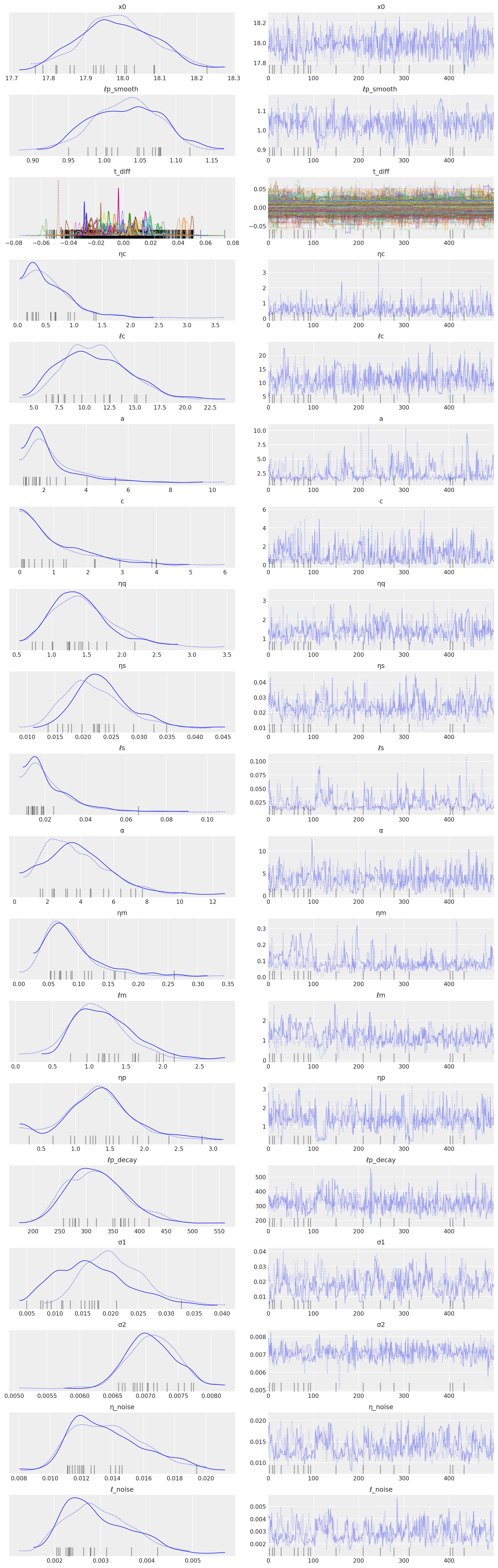
az.plot_trace(tr, compact=True);

/Users/alex_andorra/opt/anaconda3/envs/dev-pymc/lib/python3.6/site-packages/arviz/data/io_pymc3.py:89: FutureWarning: Using `from_pymc3` without the model will be deprecated in a future release. Not using the model will return less accurate and less useful results. Make sure you use the model argument or call from_pymc3 within a model context.
  FutureWarning,

tnew = np.linspace(1700, 2040, 3000) * 0.01
with model:
    fnew = gp.conditional("fnew", Xnew=tnew[:, None])

/Users/alex_andorra/tptm_alex/pymc3/pymc3/gp/cov.py:93: UserWarning: Only 1 column(s) out of Subtensor{int64}.0 are being used to compute the covariance function. If this is not intended, increase 'input_dim' parameter to the number of columns to use. Ignore otherwise.
  " the number of columns to use. Ignore otherwise.", UserWarning)

with model:
    ppc = pm.sample_posterior_predictive(tr, samples=200, var_names=["fnew"])

/Users/alex_andorra/tptm_alex/pymc3/pymc3/sampling.py:1708: UserWarning: samples parameter is smaller than nchains times ndraws, some draws and/or chains may not be represented in the returned posterior predictive sample
  "samples parameter is smaller than nchains times ndraws, some draws "

100.00% [200/200 46:10<00:00]

Below is a plot of the data since the 18th century (Mauna Loa and Law Dome ice core data) used to fit the model. The light blue lines are a bit hard to make out at this level of zoom, but they are samples from the posterior of the Gaussian process. They both interpolate the observed data, and represent plausible trajectories of the future forecast. These samples can alternatively be used to define credible intervals.

plt.figure(figsize=(12, 5))
plt.plot(tnew * 100, y_sd * ppc["fnew"][0:200:5, :].T + y_mu, color="lightblue", alpha=0.8)
plt.plot(
    [-1000, -1001],
    [-1000, -1001],
    color="lightblue",
    alpha=0.8,
    label="samples from the posterior",
)
plt.plot(t, y, "k.", label="observed data")
plt.plot(
    air_test.year.values,
    air_test.CO2.values,
    ".",
    color="orange",
    label="test set data",
)
plt.axhline(y=400, color="k", alpha=0.7, linestyle=":")
plt.ylabel("CO2 [ppm]")
plt.xlabel("year")
plt.title("fit and possible forecasts")
plt.legend()
plt.xlim([1700, 2040])
plt.ylim([260, 460]);

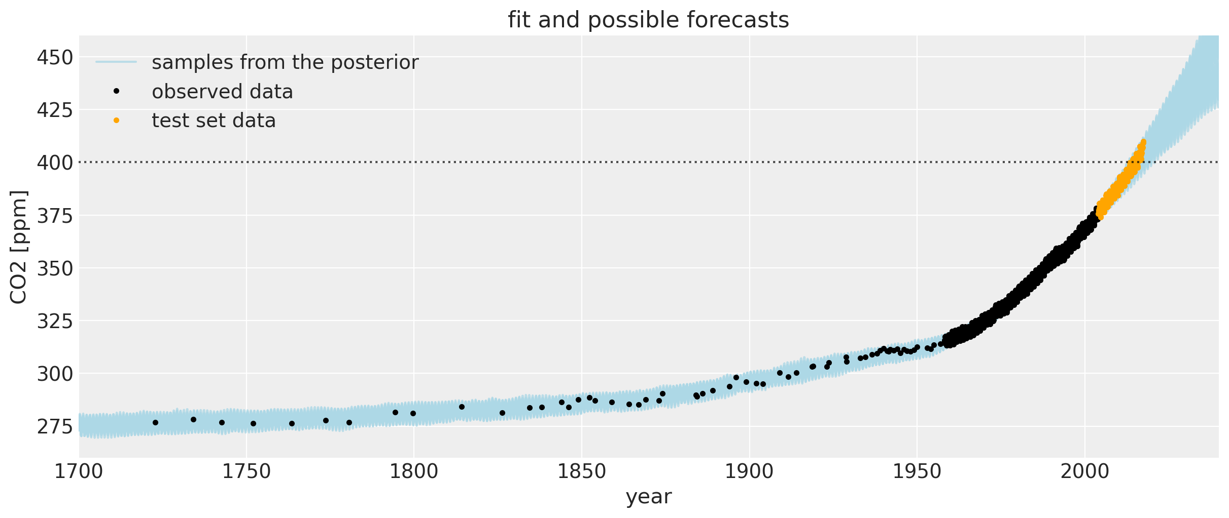
Let’s zoom in for a closer look at the uncertainty intervals at the area around when the CO2 levels first crossed 400 ppm. We can see that the posterior samples give a range of plausible future trajectories. Note that the data plotted in orange were not used in fitting the model.

plt.figure(figsize=(12, 5))
plt.plot(tnew * 100, y_sd * ppc["fnew"][0:200:5, :].T + y_mu, color="lightblue", alpha=0.8)
plt.plot(
    [-1000, -1001],
    [-1000, -1001],
    color="lightblue",
    alpha=0.8,
    label="samples from the posterior",
)
plt.plot(
    air_test.year.values,
    air_test.CO2.values,
    ".",
    color="orange",
    label="test set data",
)
plt.axhline(y=400, color="k", alpha=0.7, linestyle=":")
plt.ylabel("CO2 [ppm]")
plt.xlabel("year")
plt.title("fit and possible forecasts")
plt.legend()
plt.xlim([2004, 2040])
plt.ylim([360, 460]);

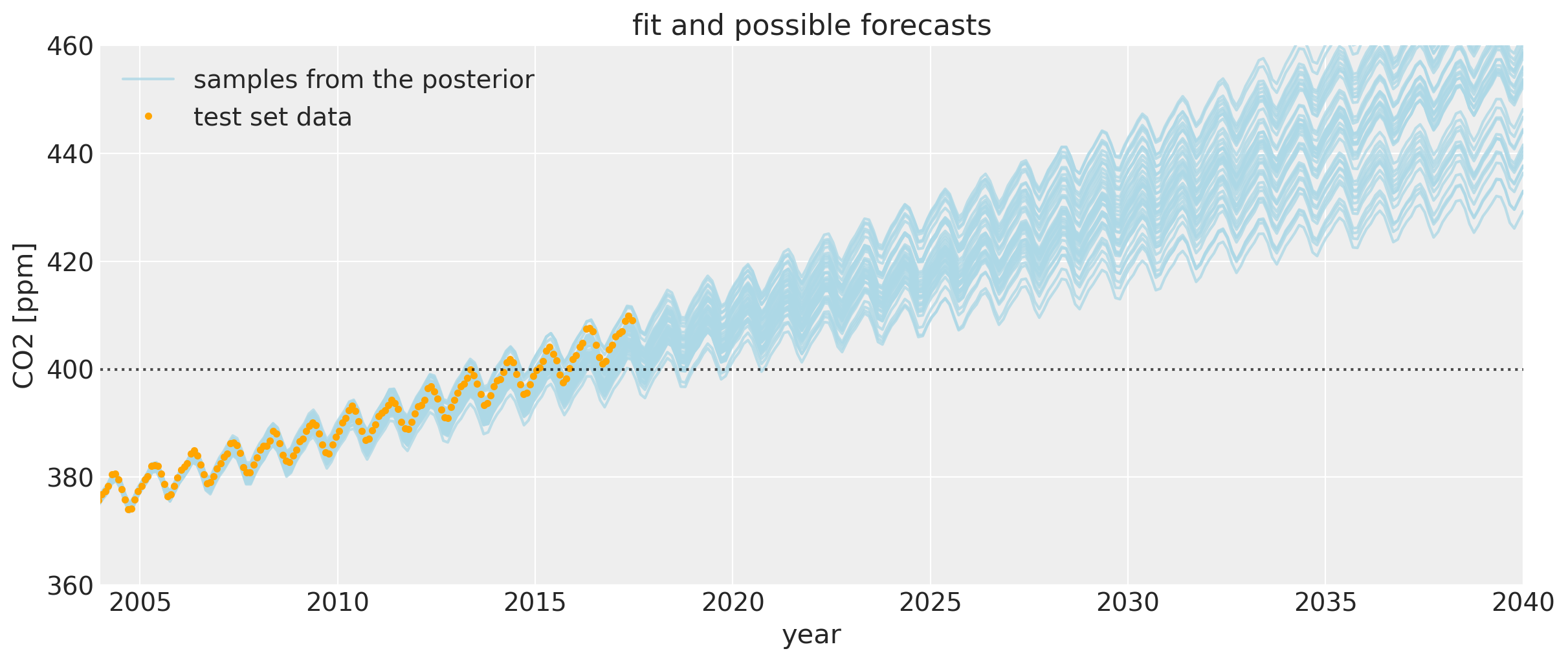
If you compare this to the first Mauna Loa example notebook, the predictions are much better. The date when the CO2 level first hits 400 is predicted much more accurately. This improvement in the bias is due to including the Polynomial * Matern52 term, and the changepoint model.

We can also look at what the model says about CO2 levels back in time. Since we allowed the x measurements to have uncertainty, we are able to fit the seasonal component back in time. To be sure, backcasting Mauna Loa CO2 measurements using ice core data doesn’t really make sense from a scientific point of view, because CO2 levels due to seasonal variation are different depending on your location on the planet. Mauna Loa will have a much more pronounced cyclical pattern because the northern hemisphere has much more vegetation. The amount of vegetation largely drives the seasonality due to the growth and die-off of plants in summers and winters. But just because it’s cool, lets look at the fit of the model here anyway:

tnew = np.linspace(11, 32, 500) * 0.01
with model:
    fnew2 = gp.conditional("fnew2", Xnew=tnew[:, None])

/Users/alex_andorra/tptm_alex/pymc3/pymc3/gp/cov.py:93: UserWarning: Only 1 column(s) out of Subtensor{int64}.0 are being used to compute the covariance function. If this is not intended, increase 'input_dim' parameter to the number of columns to use. Ignore otherwise.
  " the number of columns to use. Ignore otherwise.", UserWarning)

with model:
    ppc = pm.sample_posterior_predictive(tr, samples=200, var_names=["fnew2"])

/Users/alex_andorra/tptm_alex/pymc3/pymc3/sampling.py:1708: UserWarning: samples parameter is smaller than nchains times ndraws, some draws and/or chains may not be represented in the returned posterior predictive sample
  "samples parameter is smaller than nchains times ndraws, some draws "

100.00% [200/200 01:08<00:00]

plt.figure(figsize=(12, 5))

plt.plot(tnew * 100, y_sd * ppc["fnew2"][0:200:10, :].T + y_mu, color="lightblue", alpha=0.8)
plt.plot(
    [-1000, -1001],
    [-1000, -1001],
    color="lightblue",
    alpha=0.8,
    label="samples from the GP posterior",
)
plt.plot(100 * (t_n[:111][:, None] - tr["t_diff"].T), y[:111], "oy", alpha=0.01)
plt.plot(
    [100, 200],
    [100, 200],
    "oy",
    alpha=0.3,
    label="data location posterior samples reflecting ice core time measurement uncertainty",
)
plt.plot(t, y, "k.", label="observed data")
plt.plot(air_test.year.values, air_test.CO2.values, ".", color="orange")
plt.legend(loc="upper left")
plt.ylabel("CO2 [ppm]")
plt.xlabel("year")
plt.xlim([12, 31])
plt.xticks(np.arange(12, 32))
plt.ylim([272, 283]);

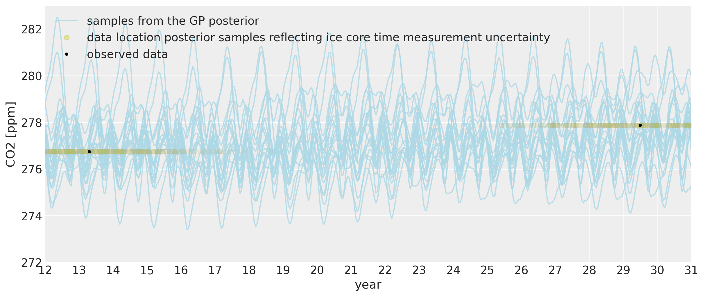
We can see that far back in time, we can backcast even the seasonal behavior to some degree. The ~two year of uncertainty in the x locations allows them to be shifted onto the nearest part of the seasonal oscillation for that year. The magnitude of the oscillation is the same as it is now in modern times. While the cycle in each of the posterior samples still has an annual period, its exact morphology is less certain since we are far in time from the dates when the Mauna Loa data was collected.

tnew = np.linspace(-20, 0, 300) * 0.01
with model:
    fnew3 = gp.conditional("fnew3", Xnew=tnew[:, None])

/Users/alex_andorra/tptm_alex/pymc3/pymc3/gp/cov.py:93: UserWarning: Only 1 column(s) out of Subtensor{int64}.0 are being used to compute the covariance function. If this is not intended, increase 'input_dim' parameter to the number of columns to use. Ignore otherwise.
  " the number of columns to use. Ignore otherwise.", UserWarning)

with model:
    ppc = pm.sample_posterior_predictive(tr, samples=200, var_names=["fnew3"])

/Users/alex_andorra/tptm_alex/pymc3/pymc3/sampling.py:1708: UserWarning: samples parameter is smaller than nchains times ndraws, some draws and/or chains may not be represented in the returned posterior predictive sample
  "samples parameter is smaller than nchains times ndraws, some draws "

100.00% [200/200 00:52<00:00]

plt.figure(figsize=(12, 5))

plt.plot(tnew * 100, y_sd * ppc["fnew3"][0:200:10, :].T + y_mu, color="lightblue", alpha=0.8)
plt.plot(
    [-1000, -1001],
    [-1000, -1001],
    color="lightblue",
    alpha=0.8,
    label="samples from the GP posterior",
)
plt.legend(loc="upper left")
plt.ylabel("CO2 [ppm]")
plt.xlabel("year")
plt.xlim([-20, 0])
plt.ylim([272, 283]);

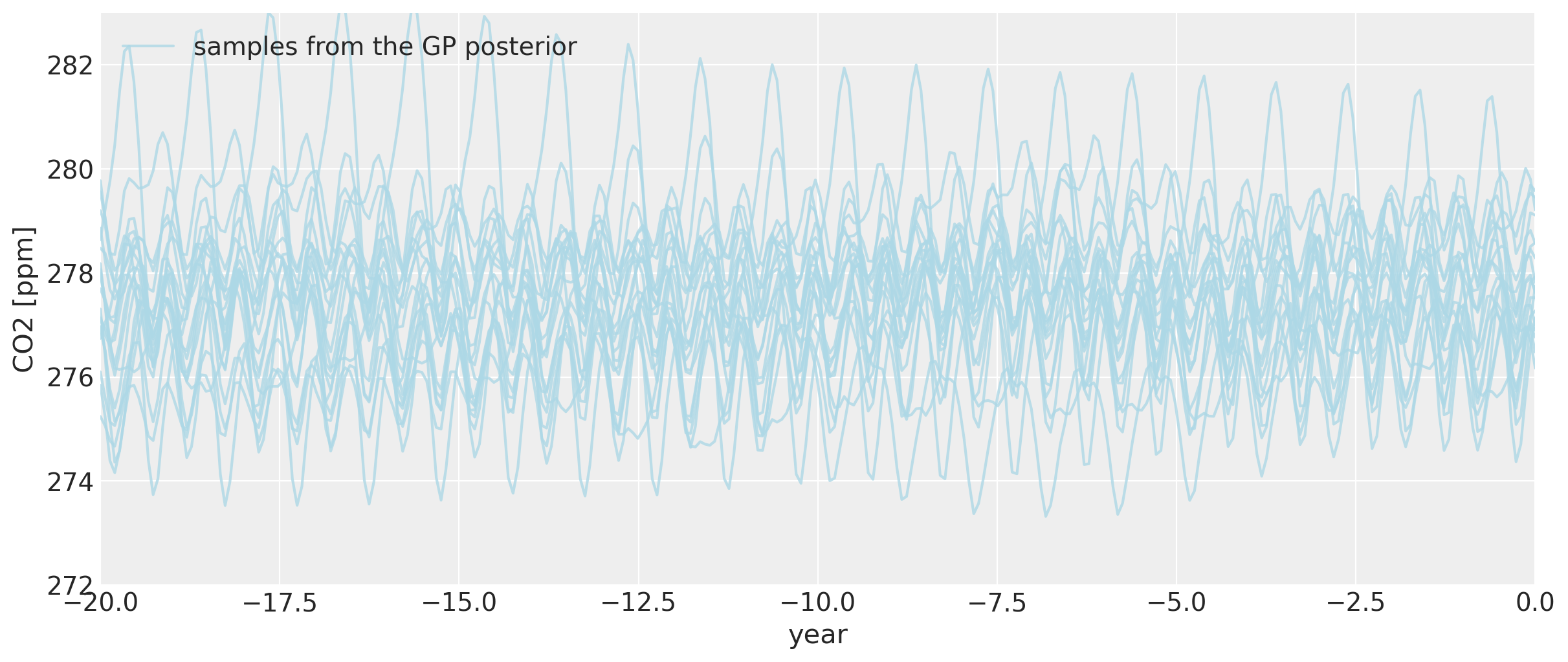
Even as we go back before the year zero BCE, the general backcasted seasonality pattern remains intact, though it does begin to vary more wildly.

Conclusion

The goal of this notebook is to help provide some ideas of ways to take advantage of the flexibility of PyMC3’s GP modeling capabilities. Data rarely comes in neat, evenly sampled intervals from a single source, which is no problem for GP models in general. To enable modeling interesting behavior, it is easy to define custom covariance and mean functions. There is no need to worry about figuring out the gradients, since this is taken care of by Theano’s autodiff capabilities. Being able to use the extremely high quality NUTS sampler in PyMC3 with GP models means that it’s possible to use samples from the posterior distribution as possible forecasts, which take into account uncertainty in the mean and covariance function hyperparameters.

%load_ext watermark
%watermark -n -u -v -iv -w

theano 1.0.5
pandas 1.1.0
numpy  1.19.1
pymc3  3.9.3
arviz  0.9.0
last updated: Sun Aug 09 2020 

CPython 3.6.11
IPython 7.16.1
watermark 2.0.2