GP-Circular

import arviz as az
import matplotlib.pyplot as plt
import numpy as np
import pymc3 as pm
import theano.tensor as tt

%config InlineBackend.figure_format = 'retina'
RANDOM_SEED = 42
np.random.seed(RANDOM_SEED)
az.style.use("arviz-darkgrid")

Circular domains are a challenge for Gaussian Processes.

• Periodic patterns are assumed, but they are hard to capture with primitives

• For circular domain \([0, \pi)\) how to model correlation between \(\pi-\varepsilon\) and \(\varepsilon\), real distance is \(2\varepsilon\), but computes differently if you just treat it non circular \((\pi-\varepsilon) - \varepsilon\)

• For correctly computed distances we need to verify kernel we obtain is positive definite

An alternative approach is required.

In the following paper, the Weinland function is used to solve the problem and ensures positive definite kernel on the circular domain (and not only).

\[ W_c(t) = \left(1 + \tau \frac{t}{c}\right)\left(1-\frac{t}{c}\right)_+^\tau \]

where \(c\) is maximum value for \(t\) and \(\tau\ge 4\) is some positive number

The kernel itself for geodesic distance (arc length) on a circle looks like

\[ k_g(x, y) = W_\pi(\text{dist}_{\mathit{geo}}(x, y)) \]

Briefly, you can think

• \(t\) is time, it runs from \(0\) to \(24\) and then goes back to \(0\)

• \(c\) is maximum distance between any timestamps, here it would be \(12\)

• \(\tau\) is proportional to the correleation strength. Let’s see how much!

In python the Weinland function is implemented like this

def weinland(t, c, tau=4):
    return (1 + tau * t / c) * np.clip(1 - t / c, 0, np.inf) ** tau

We also need implementation for the distance on a circular domain

def angular_distance(x, y, c):
    # https://stackoverflow.com/questions/1878907/the-smallest-difference-between-2-angles
    return (x - y + c) % (c * 2) - c

C = np.pi
x = np.linspace(0, C)

Let’s visualize what the Weinland function is, and how it affects the kernel:

plt.figure(figsize=(16, 9))
for tau in range(4, 10):
    plt.plot(x, weinland(x, C, tau), label=f"tau={tau}")
plt.legend()
plt.ylabel("K(x, y)")
plt.xlabel("dist");

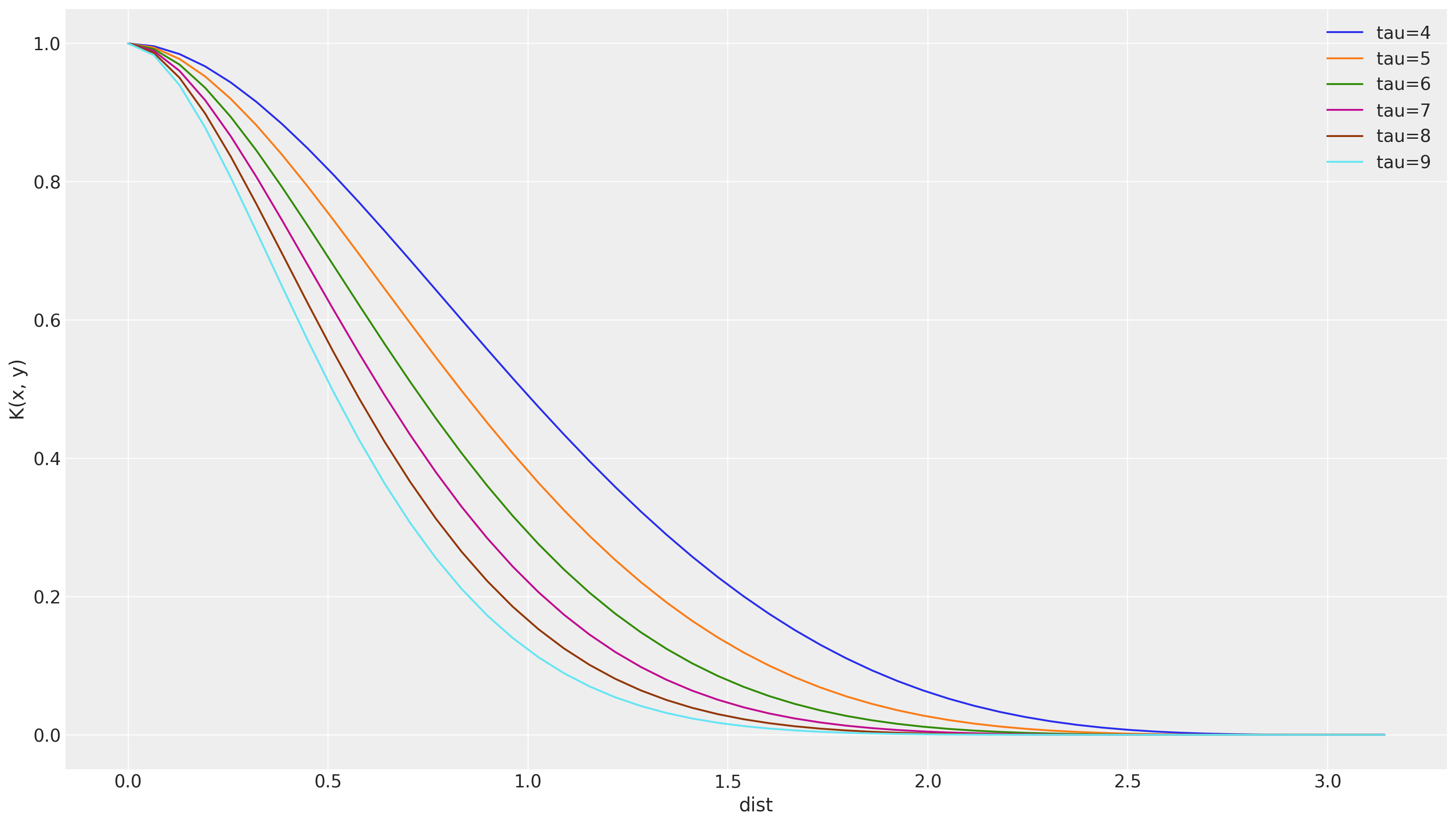
As we see, the higher \(\tau\) is, the less correlated the samples

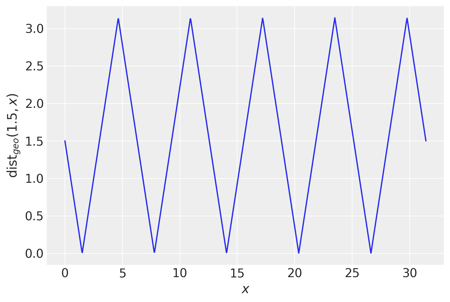
Also, let’s validate our circular distance function is working as expected

plt.plot(
    np.linspace(0, 10 * np.pi, 1000),
    abs(angular_distance(np.linspace(0, 10 * np.pi, 1000), 1.5, C)),
)
plt.ylabel(r"$\operatorname{dist}_{geo}(1.5, x)$")
plt.xlabel("$x$");

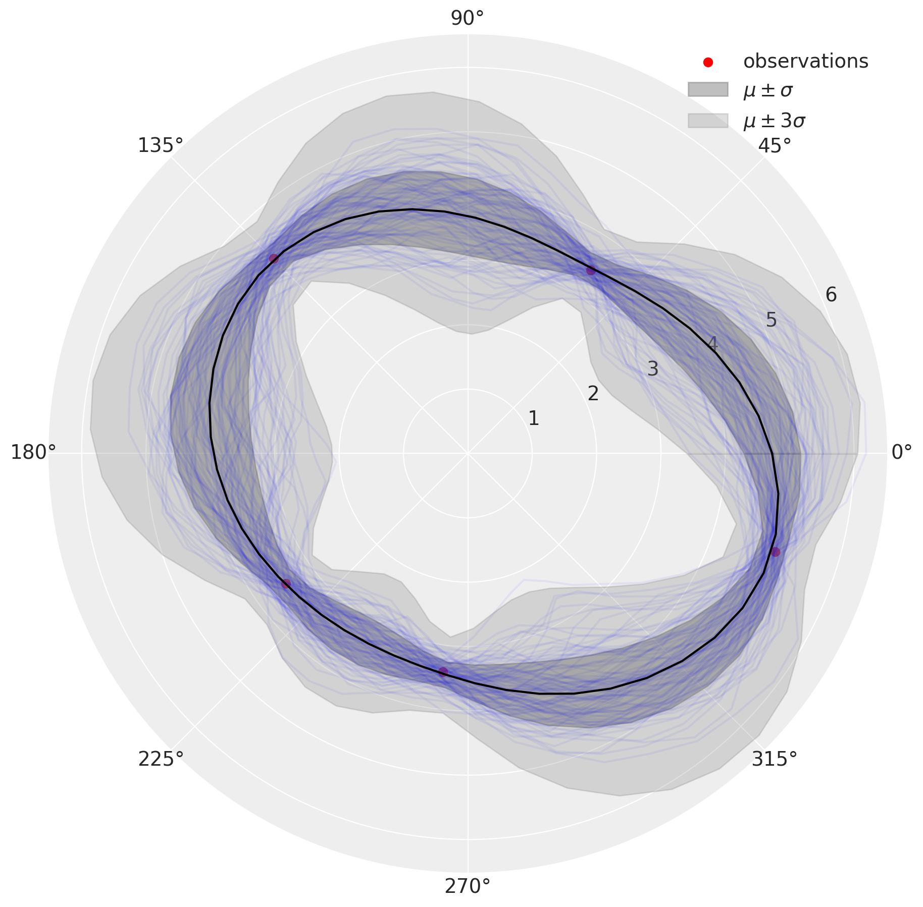
In pymc3 we will use pm.gp.cov.Circular to model circular functions

angles = np.linspace(0, 2 * np.pi)
observed = dict(x=np.random.uniform(0, np.pi * 2, size=5), y=np.random.randn(5) + 4)


def plot_kernel_results(Kernel):
    """
    To check for many kernels we leave it as a parameter
    """
    with pm.Model() as model:
        cov = Kernel()
        gp = pm.gp.Marginal(pm.gp.mean.Constant(4), cov_func=cov)
        lik = gp.marginal_likelihood("x_obs", X=observed["x"][:, None], y=observed["y"], noise=0.2)
        mp = pm.find_MAP()
        # actual functions
        y_sampled = gp.conditional("y", angles[:, None])
        # GP predictions (mu, cov)
        y_pred = gp.predict(angles[:, None], point=mp)
        trace = pm.sample_posterior_predictive([mp], var_names=["y"], samples=100)
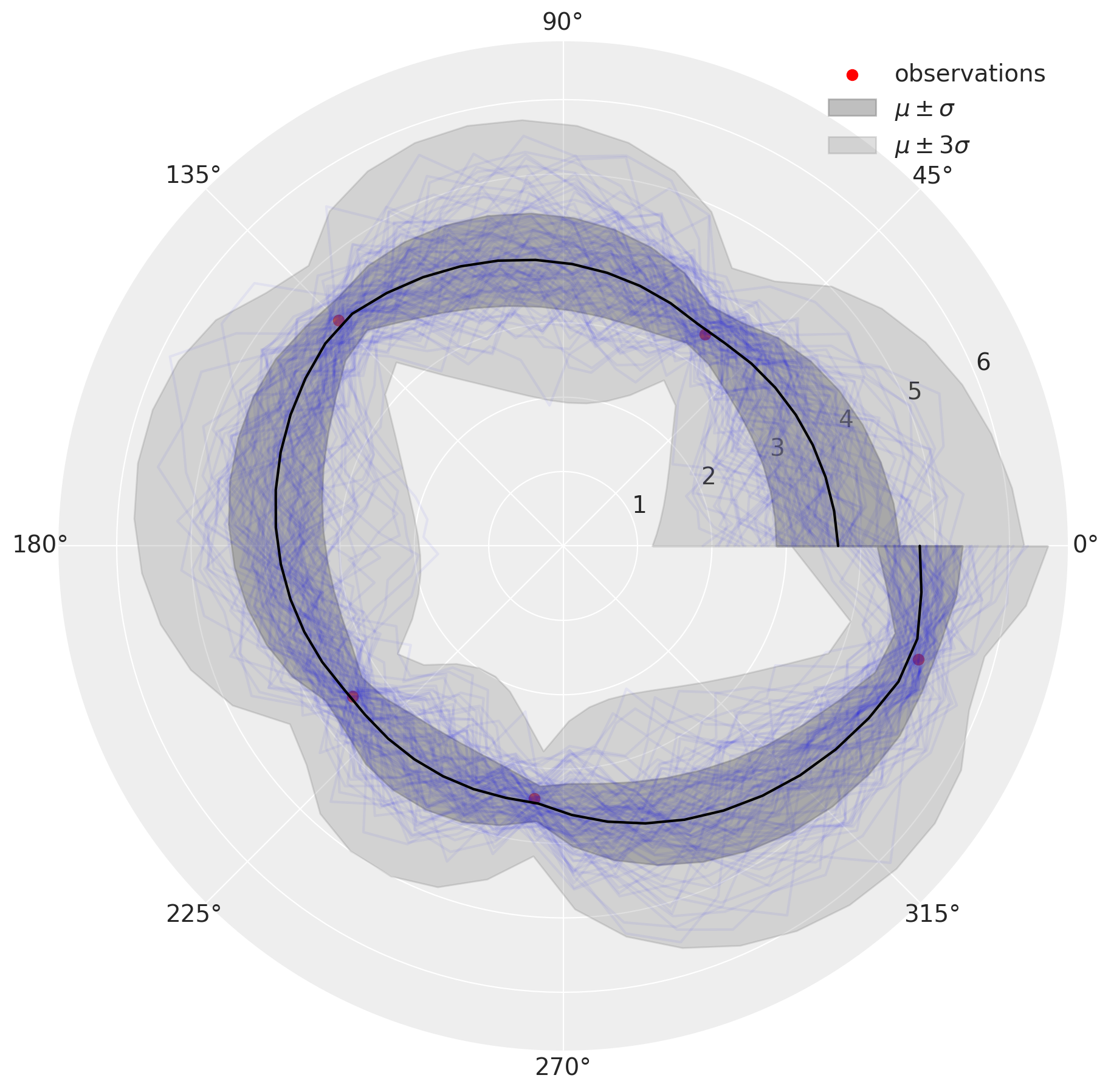
    plt.figure(figsize=(9, 9))
    paths = plt.polar(angles, trace["y"].T, color="b", alpha=0.05)
    plt.scatter(observed["x"], observed["y"], color="r", alpha=1, label="observations")
    plt.polar(angles, y_pred[0], color="black")
    plt.fill_between(
        angles,
        y_pred[0] - np.diag(y_pred[1]) ** 0.5,
        y_pred[0] + np.diag(y_pred[1]) ** 0.5,
        color="gray",
        alpha=0.5,
        label=r"$\mu\pm\sigma$",
    )
    plt.fill_between(
        angles,
        y_pred[0] - np.diag(y_pred[1]) ** 0.5 * 3,
        y_pred[0] + np.diag(y_pred[1]) ** 0.5 * 3,
        color="gray",
        alpha=0.25,
        label=r"$\mu\pm3\sigma$",
    )
    plt.legend()

def circular():
    tau = pm.Deterministic("τ", pm.Gamma("_τ", alpha=2, beta=1) + 4)
    cov = pm.gp.cov.Circular(1, period=2 * np.pi, tau=tau)
    return cov

plot_kernel_results(circular)

100.00% [7/7 00:00<00:00 logp = -6.9811, ||grad|| = 0.94385]

100.00% [100/100 00:01<00:00]

An alternative solution is Periodic kernel.

Note:

• In Periodic kernel, the key parameter to control for correlation between points is ls

• In Circular kernel it is tau, adding ls parameter did not make sense since it cancels out

Basically there is little difference between these kernels, only the way to model correlations.

def periodic():
    ls = pm.Gamma("ℓ", alpha=2, beta=1)
    return pm.gp.cov.Periodic(1, 2 * np.pi, ls=ls)

plot_kernel_results(periodic)

100.00% [13/13 00:00<00:00 logp = -7.1213, ||grad|| = 0.0066278]

100.00% [100/100 00:00<00:00]

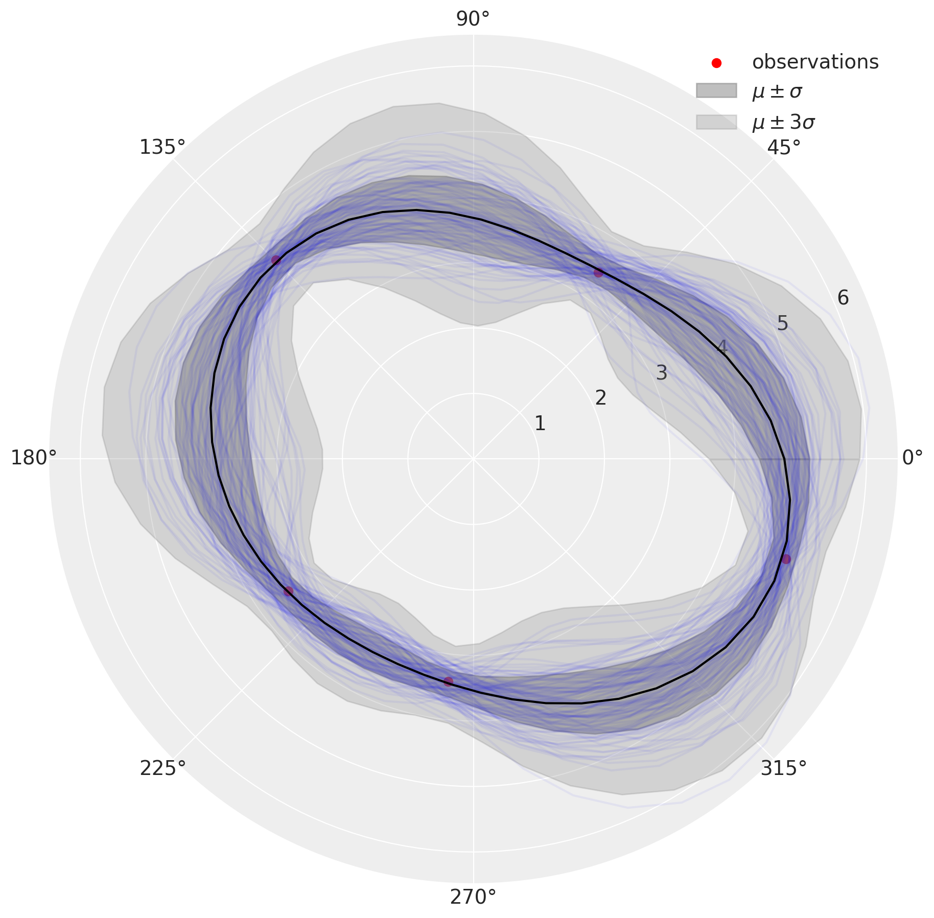
From the simulation, we see that Circular kernel leads to a more uncertain posterior.

Let’s see how Exponential kernel fails

def rbf():
    ls = pm.Gamma("ℓ", alpha=2, beta=1)
    return pm.gp.cov.Exponential(1, ls=ls)

plot_kernel_results(rbf)

100.00% [6/6 00:00<00:00 logp = -7.4099, ||grad|| = 1.8782]

100.00% [100/100 00:01<00:00]

The results look similar to what we had with Circular kernel, but the change point \(0^\circ\) is not taken in account

Conclusions

• Use circular/periodic kernel once you strongly believe function should smoothly go through the boundary of the cycle

• Periodic kernel is as fine as Circular except that the latter allows more uncertainty

• RBF kernel is not the right choice

%load_ext watermark
%watermark -n -u -v -iv -w

pymc3 3.9.3
numpy 1.19.0
arviz 0.9.0
last updated: Sat Oct 10 2020 

CPython 3.8.6
IPython 7.17.0
watermark 2.0.2