GenPareto

class pymc_extras.distributions.GenPareto(name: str, *args, rng=None, dims: str | Sequence[str | None] | None = None, initval=None, observed=None, total_size=None, transform=UNSET, default_transform=UNSET, **kwargs)

Generalized Pareto distribution.

The Generalized Pareto distribution (GPD) is the canonical model for exceedances over a threshold (peaks-over-threshold), the counterpart of the GEV used for block maxima. Its CDF is

\[\begin{split}G(x \mid \mu, \sigma, \xi) = \begin{cases} 1 - \left(1 + \xi\,\frac{x - \mu}{\sigma}\right)^{-1/\xi}, & \xi \neq 0, \\[6pt] 1 - \exp\!\left(-\dfrac{x - \mu}{\sigma}\right), & \xi = 0. \end{cases}\end{split}\]

The shape \(\xi\) is parametrized as in Scarrott and MacDonald (2012) [1], matching SciPy’s genpareto c parameter.

(Source code, png, hires.png, pdf)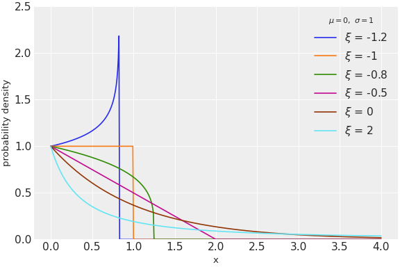

Support	\(\begin{cases} x \geq \mu, & \xi \geq 0 \\ \mu \leq x < \mu - \sigma/\xi, & \xi < 0 \end{cases}\)
Mean	\(\begin{cases} \mu + \dfrac{\sigma}{1 - \xi}, & \xi < 1 \\ \infty, & \xi \geq 1 \end{cases}\)
Variance	\(\begin{cases} \dfrac{\sigma^2}{(1 - \xi)^2 (1 - 2\xi)}, & \xi < 1/2 \\ \infty, & \xi \geq 1/2 \end{cases}\)
Median	\(\begin{cases} \mu + \dfrac{\sigma (2^{\xi} - 1)}{\xi}, & \xi \neq 0 \\ \mu + \sigma \ln 2, & \xi = 0 \end{cases}\)
Mode	\(\begin{cases} \mu, & \xi \geq -1 \\ \mu - \sigma/\xi, & \xi \leq -1 \end{cases}\)
Entropy	\(\ln \sigma + \xi + 1\)

Parameters:

• mu (tensor_like of float) – Location parameter (the threshold).

• sigma (tensor_like of float) – Scale parameter (sigma > 0).

• xi (tensor_like of float) – Shape parameter. \(\xi > 0\) gives a heavy (Pareto) tail, \(\xi = 0\) an exponential tail, and \(\xi < 0\) a bounded upper tail.

References

[1]

Scarrott, C., & MacDonald, A. (2012). A review of extreme value threshold estimation and uncertainty quantification. REVSTAT - Statistical Journal, 10(1), 33-60. https://doi.org/10.57805/revstat.v10i1.110

[2]

Pickands, J. (1975). Statistical Inference Using Extreme Order Statistics. Annals of Statistics, 3(1), 119-131. https://www.jstor.org/stable/2958083

Notes

The support is \([\mu, \infty)\) for \(\xi \geq 0\). For \(\xi < 0\), the support has a finite right endpoint \(x_F := \mu - \sigma/\xi\); values at or above \(x_F\) have density \(0\). Since \(x_F\) depends on \(\sigma\) and \(\xi\), a fit that leaves them free must keep every observation inside the support (see Modeling recommendations).

The \(r\)-th moment is finite iff \(\xi < 1/r\). Thus the mean is finite for \(\xi < 1\) and the variance for \(\xi < 1/2\). Every moment exists for \(\xi \leq 0\).

Examples

Fitting exceedances over a known threshold:

import pymc as pm
from pymc_extras.distributions import GenPareto

exceedances = data[data > threshold]
xmax = exceedances.max()
with pm.Model():
    # sigma carries the data's units; use a wide log-scale prior when the
    # data scale is unknown.
    pareto_sigma = pm.LogNormal("pareto_sigma", mu=0.0, sigma=10.0)
    # xi lower bound: see Modeling recommendations.
    pareto_xi = pm.TruncatedNormal(
        "pareto_xi",
        mu=0.0,
        sigma=2.0,
        lower=pm.math.maximum(-1.0, -pareto_sigma / (xmax - threshold)),
    )
    GenPareto("obs", mu=threshold, sigma=pareto_sigma, xi=pareto_xi, observed=exceedances)
    idata = pm.sample()

Modeling recommendations

• Keep the data inside the support. If \(\xi\) is allowed to be negative, the support has a finite upper wall \(x = x_F\), where \(x_F := \mu - \sigma/\xi\), and the observations stay inside it only when \(\max(\text{data}) < x_F\), equivalently \(\xi > -\sigma/(\max(\text{data}) - \mu)\). Encoding this as the \(\xi\) prior’s lower bound keeps \(x_F\) above the data; without it the sampler can reach \((\sigma, \xi)\) for which \(x_F < \max(\text{data})\), putting an observation out of support and causing divergences. (\(\xi \geq 0\) has no upper wall and always contains the data.)

• Floor \(\xi\) at \(-1\). If \(\xi\) is allowed below \(-1\), the density diverges at the wall \(x = x_F\): as \(x_F\) decreases toward \(\max(\text{data})\) the likelihood tends to \(+\infty\). Choose the \(\xi\) prior to enforce \(\xi \geq -1\) (where the wall density is finite); combined with the in-support bound, this gives the example prior’s lower limit \(\max(-1,\ -\sigma/(\max(\text{data}) - \mu))\).

• Cap \(\xi\) from above if moments must exist. When the application needs a finite mean or variance, bound the \(\xi\) prior above accordingly: \(\xi < 1\) (mean) or \(\xi < 1/2\) (variance).

• Keep \(\mu\) fixed at the threshold. In a peaks-over-threshold fit \(\mu\) is chosen in advance, not inferred. Estimating it has two failure modes: proposals with \(\mu > \min(\text{data})\) put observations out of support, and the corner \(\mu \to \min(\text{data})\), \(\sigma \to 0\) has unbounded likelihood when \(\xi > n - 1\).

Implementation details

Numerical precision near the wall. As \(x\) nears the wall \(x = x_F\), the margin \(1 + \xi (x - \mu)/\sigma\) cancels toward \(0\). The log-density value stays accurate, but its gradient w.r.t. \(\sigma\) and \(\xi\) has relative error of order the machine epsilon divided by that margin. It stems from the finite precision of \(x\), and no reformulation of logp avoids it.

Difference from SciPy. For \(\xi < 0\) the wall \(x = x_F\) is treated as open: logp returns \(-\infty\) there. There is a finite limiting density for \(-1 \leq \xi < 0\) as \(x \to x_F^-\), and SciPy returns the limiting value. This endpoint carries zero probability mass, so the choice affects neither sampling nor integration.

__init__()

Methods

__init__()
dist([mu, sigma, xi])	Create a tensor variable corresponding to the cls distribution.
icdf(mu, sigma, xi)
logccdf(mu, sigma, xi)
logcdf(mu, sigma, xi)
logp(mu, sigma, xi)
rv_op(mu, sigma, xi, *[, size, rng])
support_point(size, mu, sigma, xi)