ExtGenPareto

class pymc_extras.distributions.ExtGenPareto(name: str, *args, rng=None, dims: str | Sequence[str | None] | None = None, initval=None, observed=None, total_size=None, transform=UNSET, default_transform=UNSET, **kwargs)

Extended Generalized Pareto distribution.

The extended GPD (Type 1) of Naveau et al. (2016) [1] is equivalent to the EGP3 model of Papastathopoulos and Tawn (2013) [2]. It transforms the GPD CDF \(G\) through the carrier \(v \mapsto v^\kappa\):

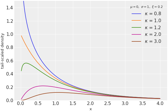
\[F(x \mid \mu, \sigma, \xi, \kappa) = \left[G\!\left(x \mid \mu, \sigma, \xi\right)\right]^{\kappa}.\]

The GPD parameters \(\mu, \sigma, \xi\) describe the tail (large \(x\)), as in the GPD. \(\kappa > 0\) is an additional shape parameter for the body (small \(x\)); \(\kappa = 1\) recovers the GPD. The extra parameter gives more flexibility to model the body while leaving the GPD tail unchanged. Typical applications include threshold exceedances [2] and modeling rainfall intensities [1].

(Source code, png, hires.png, pdf)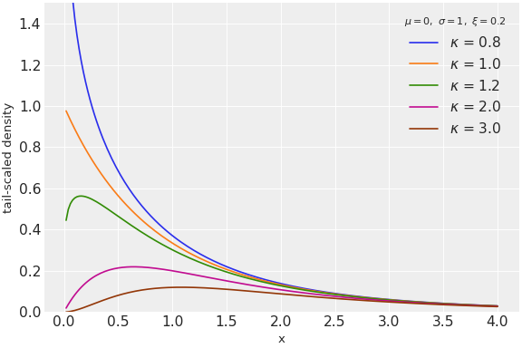

Support	\(\begin{cases} x \geq \mu, & \xi \geq 0 \\ \mu \leq x < \mu - \sigma/\xi, & \xi < 0 \end{cases}\)
Mean	\(\begin{cases} \mu + \dfrac{\sigma}{\xi}\left[\kappa B(\kappa, 1 - \xi) - 1\right], & \xi < 1,\ \xi \neq 0 \\ \mu + \sigma\left(\psi(\kappa + 1) + \gamma\right), & \xi = 0 \\ \infty, & \xi \geq 1 \end{cases}\)
Variance	\(\begin{cases} \left(\dfrac{\sigma}{\xi}\right)^2 \left[\kappa B(\kappa, 1 - 2\xi) - \kappa^2 B(\kappa, 1 - \xi)^2\right], & \xi < 1/2,\ \xi \neq 0 \\ \sigma^2\left(\pi^2/6 - \psi'(\kappa + 1)\right), & \xi = 0 \\ \infty, & \xi \geq 1/2 \end{cases}\)
Median	\(\begin{cases} \mu + \dfrac{\sigma}{\xi}\left[\left(1 - 2^{-1/\kappa}\right)^{-\xi} - 1\right], & \xi \neq 0 \\ \mu - \sigma\ln\!\left(1 - 2^{-1/\kappa}\right), & \xi = 0 \end{cases}\)
Mode	\(\begin{cases} \mu + \dfrac{\sigma}{\xi}\left(T^{-\xi} - 1\right), & \kappa > 1,\ \xi \geq -1,\ \xi \neq 0 \\ \mu + \sigma\ln\kappa, & \kappa > 1,\ \xi = 0 \\ \mu, & \kappa \leq 1,\ \xi \geq -1 \\ \mu - \sigma/\xi, & \kappa \geq 1,\ \xi < -1 \end{cases}\) where \(T = \dfrac{1 + \xi}{\kappa + \xi}\)

Here \(B(a, b) = \Gamma(a)\Gamma(b)/\Gamma(a + b)\) is the Beta function, \(\psi\) the digamma, \(\psi'\) the trigamma, and \(\gamma\) the Euler–Mascheroni constant.

Parameters:

• mu (tensor_like of float) – Location parameter (the threshold).

• sigma (tensor_like of float) – Scale parameter (sigma > 0).

• xi (tensor_like of float) – Tail shape parameter (large \(x\)), as in GenPareto.

• kappa (tensor_like of float) – Body shape parameter (small \(x\), kappa > 0). kappa = 1 reduces the distribution to GenPareto.

References

[1] (1,2)

Naveau, P., Huser, R., Ribereau, P., & Hannart, A. (2016). Modeling jointly low, moderate, and heavy rainfall intensities without a threshold selection. Water Resources Research, 52(4), 2753-2769. https://doi.org/10.1002/2015WR018552

[2] (1,2)

Papastathopoulos, I., & Tawn, J. A. (2013). Extended generalised Pareto models for tail estimation. Journal of Statistical Planning and Inference, 143(1), 131-143. https://arxiv.org/abs/1111.6899

Notes

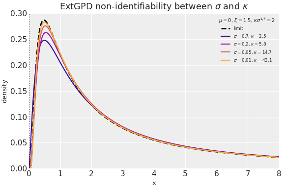
All of the Notes on GenPareto apply here too. The \(r\)-th moment is finite iff \(\xi < 1/r\), as for the GPD.

For positive \(\xi\), tail-only data can make \(\sigma\) and \(\kappa\) hard to identify separately. In the small-\(\sigma\), large-\(\kappa\) regime, observations above the threshold are informed mainly by a combined tail-survival scale rather than by the two parameters individually, making the fit sensitive to very broad \(\sigma\) priors.

(Source code, png, hires.png, pdf)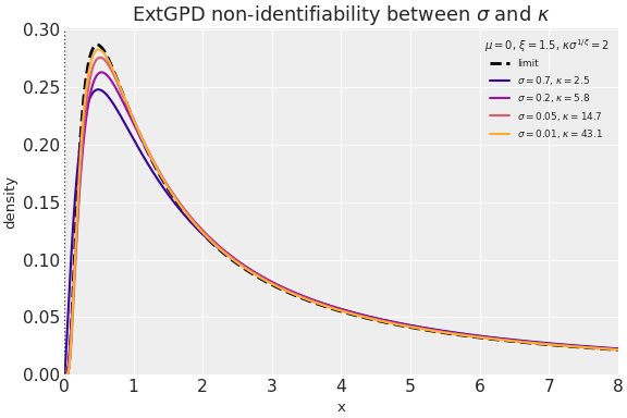

Examples

Fitting exceedances over a known threshold, with \(\kappa\) as an additional body shape:

import numpy as np
import pymc as pm
from pymc_extras.distributions import ExtGenPareto

exceedances = data[data > threshold]
xmax = exceedances.max()
excess = exceedances - threshold
s_hat = np.median(excess) / np.log(2.0)

with pm.Model():
    # Regularize sigma to the observed excess scale; see recommendations.
    pareto_sigma = pm.LogNormal("pareto_sigma", mu=np.log(s_hat), sigma=1.0)
    # Center kappa on the GPD case while allowing broad body-shape variation.
    pareto_kappa = pm.LogNormal("pareto_kappa", mu=0.0, sigma=1.0)
    # xi lower bound: see modeling recommendations below.
    pareto_xi = pm.TruncatedNormal(
        "pareto_xi",
        mu=0.0,
        sigma=2.0,
        lower=pm.math.maximum(-1.0, -pareto_sigma / (xmax - threshold)),
    )
    ExtGenPareto(
        "obs",
        mu=threshold,
        sigma=pareto_sigma,
        xi=pareto_xi,
        kappa=pareto_kappa,
        observed=exceedances,
    )
    idata = pm.sample()

Modeling recommendations

For \(\xi\), use the same lower-bound rule as GenPareto: combine the data-in-support constraint with the \(-1\) floor.

• Regularize \(\sigma\) to the excess scale. \(\sigma\) carries the data’s units, so center its prior on the observed excess scale rather than on an arbitrary unit scale. A simple closed-form default is \(\hat{s}=\operatorname{median}(x-\mu)/\log 2\), the median match for the exponential GPD carrier (\(\xi=0\), \(\kappa=1\)), with LogNormal(log(s_hat), 1). This gives a wide prior on the observed scale without encouraging the small-\(\sigma\), large-\(\kappa\) trade described in the Notes.

• Center \(\kappa\) on the GPD case. LogNormal(0, 1) is symmetric in \(\log\kappa\) about \(\kappa = 1\) and allows a broad range of body shapes while enforcing \(\kappa\) positive. \(\kappa\) is mainly informed by the body of the exceedance distribution; tail-dominated data can leave it correlated with \(\sigma\). Inspect its posterior and prefer the GPD when \(\kappa\) remains compatible with \(1\).

• Keep \(\mu\) fixed at the threshold. In a peaks-over-threshold fit, \(\mu\) is chosen in advance. Estimating it is especially unstable for ExtGPD because a \(\kappa < 1\) density diverges at the lower endpoint \(x = \mu\). If \(\mu\) must be estimated, floor \(\kappa \geq 1\) or put a prior on \(\min(\text{data}) - \mu\) that vanishes at \(0\).

__init__()

Methods

__init__()
dist([mu, sigma, xi, kappa])	Create a tensor variable corresponding to the cls distribution.
icdf(mu, sigma, xi, kappa)
logccdf(mu, sigma, xi, kappa)
logcdf(mu, sigma, xi, kappa)
logp(mu, sigma, xi, kappa)
rv_op(mu, sigma, xi, kappa, *[, size, rng])
support_point(size, mu, sigma, xi, kappa)