GLM: Mini-batch ADVI on hierarchical regression model

Unlike Gaussian mixture models, (hierarchical) regression models have independent variables. These variables affect the likelihood function, but are not random variables. When using mini-batch, we should take care of that.

%env THEANO_FLAGS=device=cpu, floatX=float32, warn_float64=ignore

import os

import arviz as az
import matplotlib.pyplot as plt
import numpy as np
import pandas as pd
import pymc3 as pm
import seaborn as sns
import theano
import theano.tensor as tt

from scipy import stats

print(f"Running on PyMC3 v{pm.__version__}")

env: THEANO_FLAGS=device=cpu, floatX=float32, warn_float64=ignore
Running on PyMC3 v3.11.2

%config InlineBackend.figure_format = 'retina'
RANDOM_SEED = 8927
rng = np.random.default_rng(RANDOM_SEED)
az.style.use("arviz-darkgrid")

try:
    data = pd.read_csv(os.path.join("..", "data", "radon.csv"))
except FileNotFoundError:
    data = pd.read_csv(pm.get_data("radon.csv"))

data

	Unnamed: 0	idnum	state	state2	stfips	zip	region	typebldg	floor	room	...	pcterr	adjwt	dupflag	zipflag	cntyfips	county	fips	Uppm	county_code	log_radon
0	0	5081.0	MN	MN	27.0	55735	5.0	1.0	1.0	3.0	...	9.7	1146.499190	1.0	0.0	1.0	AITKIN	27001.0	0.502054	0	0.832909
1	1	5082.0	MN	MN	27.0	55748	5.0	1.0	0.0	4.0	...	14.5	471.366223	0.0	0.0	1.0	AITKIN	27001.0	0.502054	0	0.832909
2	2	5083.0	MN	MN	27.0	55748	5.0	1.0	0.0	4.0	...	9.6	433.316718	0.0	0.0	1.0	AITKIN	27001.0	0.502054	0	1.098612
3	3	5084.0	MN	MN	27.0	56469	5.0	1.0	0.0	4.0	...	24.3	461.623670	0.0	0.0	1.0	AITKIN	27001.0	0.502054	0	0.095310
4	4	5085.0	MN	MN	27.0	55011	3.0	1.0	0.0	4.0	...	13.8	433.316718	0.0	0.0	3.0	ANOKA	27003.0	0.428565	1	1.163151
...	...	...	...	...	...	...	...	...	...	...	...	...	...	...	...	...	...	...	...	...	...
914	914	5995.0	MN	MN	27.0	55363	5.0	1.0	0.0	4.0	...	4.5	1146.499190	0.0	0.0	171.0	WRIGHT	27171.0	0.913909	83	1.871802
915	915	5996.0	MN	MN	27.0	55376	5.0	1.0	0.0	7.0	...	8.3	1105.956867	0.0	0.0	171.0	WRIGHT	27171.0	0.913909	83	1.526056
916	916	5997.0	MN	MN	27.0	55376	5.0	1.0	0.0	4.0	...	5.2	1214.922779	0.0	0.0	171.0	WRIGHT	27171.0	0.913909	83	1.629241
917	917	5998.0	MN	MN	27.0	56297	5.0	1.0	0.0	4.0	...	9.6	1177.377355	0.0	0.0	173.0	YELLOW MEDICINE	27173.0	1.426590	84	1.335001
918	918	5999.0	MN	MN	27.0	56297	5.0	1.0	0.0	4.0	...	8.0	1214.922779	0.0	0.0	173.0	YELLOW MEDICINE	27173.0	1.426590	84	1.098612

919 rows × 30 columns

county_idx = data["county_code"].values
floor_idx = data["floor"].values
log_radon_idx = data["log_radon"].values

coords = {"counties": data.county.unique()}

Here, log_radon_idx_t is a dependent variable, while floor_idx_t and county_idx_t determine the independent variable.

log_radon_idx_t = pm.Minibatch(log_radon_idx, 100)
floor_idx_t = pm.Minibatch(floor_idx, 100)
county_idx_t = pm.Minibatch(county_idx, 100)

/home/ada/.local/lib/python3.8/site-packages/pymc3/data.py:316: FutureWarning: Using a non-tuple sequence for multidimensional indexing is deprecated; use `arr[tuple(seq)]` instead of `arr[seq]`. In the future this will be interpreted as an array index, `arr[np.array(seq)]`, which will result either in an error or a different result.
  self.shared = theano.shared(data[in_memory_slc])
/home/ada/.local/lib/python3.8/site-packages/pymc3/data.py:316: FutureWarning: Using a non-tuple sequence for multidimensional indexing is deprecated; use `arr[tuple(seq)]` instead of `arr[seq]`. In the future this will be interpreted as an array index, `arr[np.array(seq)]`, which will result either in an error or a different result.
  self.shared = theano.shared(data[in_memory_slc])

with pm.Model(coords=coords) as hierarchical_model:
    # Hyperpriors for group nodes
    mu_a = pm.Normal("mu_alpha", mu=0.0, sigma=100 ** 2)
    sigma_a = pm.Uniform("sigma_alpha", lower=0, upper=100)
    mu_b = pm.Normal("mu_beta", mu=0.0, sigma=100 ** 2)
    sigma_b = pm.Uniform("sigma_beta", lower=0, upper=100)

Intercept for each county, distributed around group mean mu_a. Above we just set mu and sd to a fixed value while here we plug in a common group distribution for all a and b (which are vectors with the same length as the number of unique counties in our example).

with hierarchical_model:

    a = pm.Normal("alpha", mu=mu_a, sigma=sigma_a, dims="counties")
    # Intercept for each county, distributed around group mean mu_a
    b = pm.Normal("beta", mu=mu_b, sigma=sigma_b, dims="counties")

Model prediction of radon level a[county_idx] translates to a[0, 0, 0, 1, 1, ...], we thus link multiple household measures of a county to its coefficients.

with hierarchical_model:

    radon_est = a[county_idx_t] + b[county_idx_t] * floor_idx_t

Finally, we specify the likelihood:

with hierarchical_model:

    # Model error
    eps = pm.Uniform("eps", lower=0, upper=100)

    # Data likelihood
    radon_like = pm.Normal(
        "radon_like", mu=radon_est, sigma=eps, observed=log_radon_idx_t, total_size=len(data)
    )

Random variables radon_like, associated with log_radon_idx_t, should be given to the function for ADVI to denote that as observations in the likelihood term.

On the other hand, minibatches should include the three variables above.

Then, run ADVI with mini-batch.

with hierarchical_model:
    approx = pm.fit(100000, callbacks=[pm.callbacks.CheckParametersConvergence(tolerance=1e-4)])
    idata_advi = az.from_pymc3(approx.sample(500))

/home/ada/.local/lib/python3.8/site-packages/theano/gpuarray/dnn.py:192: UserWarning: Your cuDNN version is more recent than Theano. If you encounter problems, try updating Theano or downgrading cuDNN to a version >= v5 and <= v7.
  warnings.warn(

100.00% [100000/100000 00:17<00:00 Average Loss = 120.22]

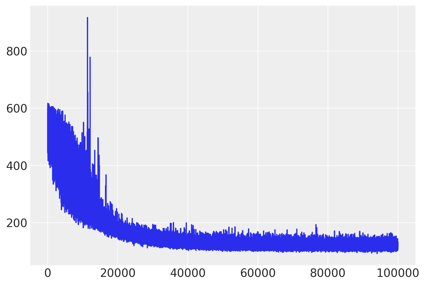
Finished [100%]: Average Loss = 120.26

Check the trace of ELBO and compare the result with MCMC.

plt.plot(approx.hist);

# Inference button (TM)!
with pm.Model(coords=coords):

    mu_a = pm.Normal("mu_alpha", mu=0.0, sigma=100 ** 2)
    sigma_a = pm.Uniform("sigma_alpha", lower=0, upper=100)
    mu_b = pm.Normal("mu_beta", mu=0.0, sigma=100 ** 2)
    sigma_b = pm.Uniform("sigma_beta", lower=0, upper=100)

    a = pm.Normal("alpha", mu=mu_a, sigma=sigma_a, dims="counties")
    b = pm.Normal("beta", mu=mu_b, sigma=sigma_b, dims="counties")

    # Model error
    eps = pm.Uniform("eps", lower=0, upper=100)

    radon_est = a[county_idx] + b[county_idx] * floor_idx

    radon_like = pm.Normal("radon_like", mu=radon_est, sigma=eps, observed=log_radon_idx)

    # essentially, this is what init='advi' does
    step = pm.NUTS(scaling=approx.cov.eval(), is_cov=True)
    hierarchical_trace = pm.sample(
        2000, step, start=approx.sample()[0], progressbar=True, return_inferencedata=True
    )

Multiprocess sampling (4 chains in 4 jobs)
NUTS: [eps, beta, alpha, sigma_beta, mu_beta, sigma_alpha, mu_alpha]

100.00% [12000/12000 11:00<00:00 Sampling 4 chains, 522 divergences]

Sampling 4 chains for 1_000 tune and 2_000 draw iterations (4_000 + 8_000 draws total) took 661 seconds.
There were 281 divergences after tuning. Increase `target_accept` or reparameterize.
There were 41 divergences after tuning. Increase `target_accept` or reparameterize.
There were 156 divergences after tuning. Increase `target_accept` or reparameterize.
There were 44 divergences after tuning. Increase `target_accept` or reparameterize.
The estimated number of effective samples is smaller than 200 for some parameters.

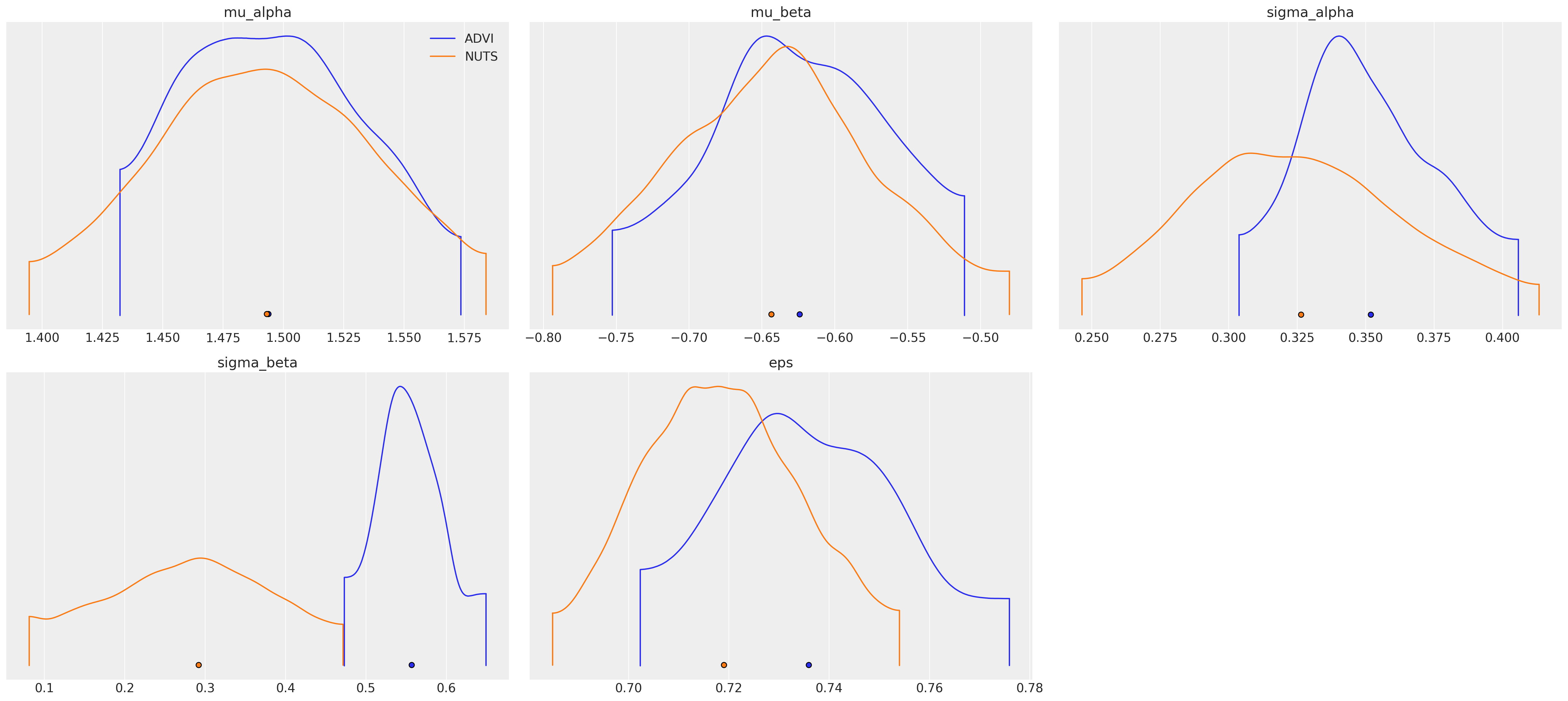
az.plot_density(
    [idata_advi, hierarchical_trace], var_names=["~alpha", "~beta"], data_labels=["ADVI", "NUTS"]
);

Watermark

%load_ext watermark
%watermark -n -u -v -iv -w -p xarray

Last updated: Thu Sep 23 2021

Python implementation: CPython
Python version       : 3.8.10
IPython version      : 7.25.0

xarray: 0.17.0

numpy     : 1.21.0
seaborn   : 0.11.1
pandas    : 1.2.1
matplotlib: 3.3.4
theano    : 1.1.2
pymc3     : 3.11.2
scipy     : 1.7.1
arviz     : 0.11.2

Watermark: 2.2.0

• PyMC Contributors . "GLM: Mini-batch ADVI on hierarchical regression model". In: PyMC Examples. Ed. by PyMC Team. DOI: 10.5281/zenodo.5832070