


Using shared variables (Data container adaptation)
import arviz as az
import matplotlib.pyplot as plt
import numpy as np
import pandas as pd
import pymc3 as pm

from numpy.random import default_rng

print(f"Running on PyMC3 v{pm.__version__}")
Running on PyMC3 v3.11.4
%matplotlib inline
%config InlineBackend.figure_format = 'retina'
RANDOM_SEED = 8927
rng = default_rng(RANDOM_SEED)
az.style.use("arviz-darkgrid")
The Data class
The pymc.Data container class wraps the theano shared variable class and lets the model be aware of its inputs and outputs. This allows one to change the value of an observed variable to predict or refit on new data. All variables of this class must be declared inside a model context and specify a name for them.
In the following example, this is demonstrated with fictional temperature observations.
df_data = pd.DataFrame(columns=["date"]).set_index("date")
dates = pd.date_range(start="2020-05-01", end="2020-05-20")

for city, mu in {"Berlin": 15, "San Marino": 18, "Paris": 16}.items():
    df_data[city] = rng.normal(loc=mu, size=len(dates))

df_data.index = dates
df_data.index.name = "date"
df_data.head()
| Berlin | San Marino | Paris | |
|---|---|---|---|
| date | |||
| 2020-05-01 | 14.777358 | 18.512741 | 14.971224 |
| 2020-05-02 | 16.325659 | 16.938007 | 15.612136 |
| 2020-05-03 | 14.429030 | 17.901775 | 15.835249 |
| 2020-05-04 | 15.668249 | 18.389226 | 16.027941 |
| 2020-05-05 | 16.145381 | 16.044643 | 17.492074 |
PyMC3 can also keep track of the dimensions (like dates or cities) and coordinates (such as the actual date times or city names) of multi-dimensional data. That way, when wraping your data around the Data container when building your model, you can specify the dimension names and coordinates of random variables, instead of specifying the shapes of those random variables as numbers.
More generally, there are two ways to specify new dimensions and their coordinates:
Entering the dimensions in the
dimskwarg of apm.Datavariable with a pandas Series or DataFrame. The name of the index and columns will be remembered as the dimensions, and PyMC3 will infer that the values of the given columns must be the coordinates.Using the new
coordsargument topymc.Modelto set the coordinates explicitly.
For more explanation about dimensions, coordinates and their big benefits, we encourage you to take a look at the ArviZ documentation.
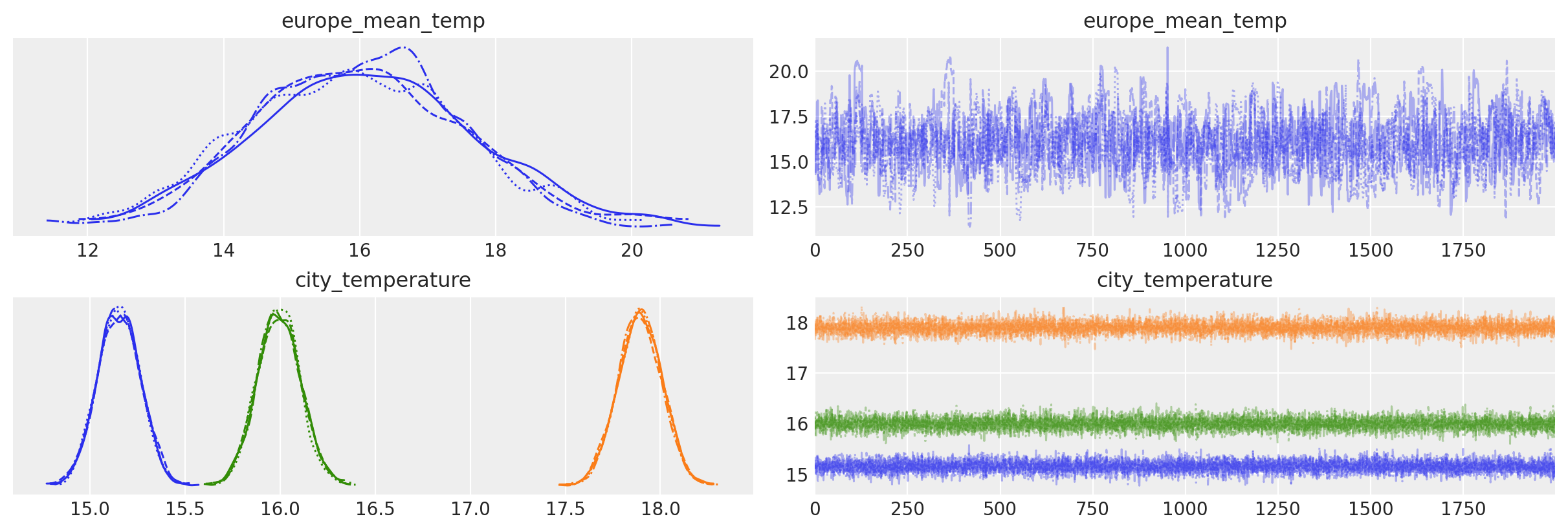
This is a lot of explanation – let’s see how it’s done! We will use a hierarchical model: it assumes a mean temperature for the European continent and models each city relative to the continent mean:
# The data has two dimensions: date and city
coords = {"date": df_data.index, "city": df_data.columns}
with pm.Model(coords=coords) as model:
    europe_mean = pm.Normal("europe_mean_temp", mu=15.0, sigma=3.0)
    city_offset = pm.Normal("city_offset", mu=0.0, sigma=3.0, dims="city")
    city_temperature = pm.Deterministic("city_temperature", europe_mean + city_offset, dims="city")

    data = pm.Data("data", df_data, dims=("date", "city"))
    pm.Normal("likelihood", mu=city_temperature, sigma=0.5, observed=data)

    idata = pm.sample(
        2000,
        tune=2000,
        target_accept=0.85,
        return_inferencedata=True,
        random_seed=RANDOM_SEED,
    )
Auto-assigning NUTS sampler...
Initializing NUTS using jitter+adapt_diag...
Multiprocess sampling (4 chains in 4 jobs)
NUTS: [city_offset, europe_mean_temp]
Sampling 4 chains for 2_000 tune and 2_000 draw iterations (8_000 + 8_000 draws total) took 42 seconds.
The number of effective samples is smaller than 10% for some parameters.
We can plot the digraph for our model using:
pm.model_to_graphviz(model)

And we see that the model did remember the coords we gave it:
model.coords
{'date': DatetimeIndex(['2020-05-01', '2020-05-02', '2020-05-03', '2020-05-04',
                '2020-05-05', '2020-05-06', '2020-05-07', '2020-05-08',
                '2020-05-09', '2020-05-10', '2020-05-11', '2020-05-12',
                '2020-05-13', '2020-05-14', '2020-05-15', '2020-05-16',
                '2020-05-17', '2020-05-18', '2020-05-19', '2020-05-20'],
               dtype='datetime64[ns]', name='date', freq='D'),
 'city': Index(['Berlin', 'San Marino', 'Paris'], dtype='object')}
Coordinates are automatically stored into the arviz.InferenceData object:
idata.posterior.coords
Coordinates:
  * chain    (chain) int64 0 1 2 3
  * draw     (draw) int64 0 1 2 3 4 5 6 7 ... 1993 1994 1995 1996 1997 1998 1999
  * city     (city) object 'Berlin' 'San Marino' 'Paris'
az.plot_trace(idata, var_names=["europe_mean_temp", "city_temperature"]);
We can get the data container variable from the model using:
model["data"].get_value()
array([[14.77735778, 18.51274112, 14.97122433],
       [16.32565874, 16.93800681, 15.61213579],
       [14.42902998, 17.90177483, 15.83524901],
       [15.6682492 , 18.38922566, 16.02794133],
       [16.14538102, 16.04464324, 17.49207391],
       [15.58734406, 18.33735625, 15.10719496],
       [14.94855671, 18.47742834, 15.59602844],
       [13.15495206, 16.89672523, 16.37053056],
       [14.69277964, 17.50128576, 16.18221169],
       [14.98823944, 18.9157944 , 17.35578274],
       [15.63543926, 17.36774846, 16.06602347],
       [15.11328912, 18.52343605, 14.85216414],
       [16.41879627, 18.38268978, 17.20631292],
       [15.79941587, 18.17817512, 16.29378664],
       [14.57242044, 17.24418161, 15.75391432],
       [16.53468809, 17.17038575, 16.86234979],
       [12.77264124, 18.54596355, 16.93790114],
       [15.28241532, 19.29121212, 16.04664653],
       [13.87844962, 18.49681212, 14.81167628],
       [16.30086967, 16.76326259, 14.47416939]])
Note that we used a theano method theano.compile.sharedvalue.SharedVariable.get_value() of class theano.compile.sharedvalue.SharedVariable to get the value of the variable. This is because our variable is actually a SharedVariable.
type(data)
theano.tensor.sharedvar.TensorSharedVariable
The methods and functions related to the Data container class are:
data_container.get_value(method inherited from the theano SharedVariable): gets the value associated with thedata_container.data_container.set_value(method inherited from the theano SharedVariable): sets the value associated with thedata_container.pymc.set_data(): PyMC3 function that sets the value associated with each Data container variable indicated in the dictionarynew_datawith it corresponding new value.
Using Data container variables to fit the same model to several datasets
This and the next sections are an adaptation of the notebook “Advanced usage of Theano in PyMC3” using pm.Data.
We can use Data container variables in PyMC3 to fit the same model to several datasets without the need to recreate the model each time (which can be time consuming if the number of datasets is large):
# We generate 10 datasets
true_mu = [rng.random() for _ in range(10)]
observed_data = [mu + rng.random(20) for mu in true_mu]

with pm.Model() as model:
    data = pm.Data("data", observed_data[0])
    mu = pm.Normal("mu", 0, 10)
    pm.Normal("y", mu=mu, sigma=1, observed=data)

# Generate one trace for each dataset
traces = []
for data_vals in observed_data:
    with model:
        # Switch out the observed dataset
        pm.set_data({"data": data_vals})
        traces.append(pm.sample(return_inferencedata=True))
Auto-assigning NUTS sampler...
Initializing NUTS using jitter+adapt_diag...
Multiprocess sampling (4 chains in 4 jobs)
NUTS: [mu]
Sampling 4 chains for 1_000 tune and 1_000 draw iterations (4_000 + 4_000 draws total) took 5 seconds.
Auto-assigning NUTS sampler...
Initializing NUTS using jitter+adapt_diag...
Multiprocess sampling (4 chains in 4 jobs)
NUTS: [mu]
Sampling 4 chains for 1_000 tune and 1_000 draw iterations (4_000 + 4_000 draws total) took 5 seconds.
Auto-assigning NUTS sampler...
Initializing NUTS using jitter+adapt_diag...
Multiprocess sampling (4 chains in 4 jobs)
NUTS: [mu]
Sampling 4 chains for 1_000 tune and 1_000 draw iterations (4_000 + 4_000 draws total) took 6 seconds.
The acceptance probability does not match the target. It is 0.8846602862032664, but should be close to 0.8. Try to increase the number of tuning steps.
Auto-assigning NUTS sampler...
Initializing NUTS using jitter+adapt_diag...
Multiprocess sampling (4 chains in 4 jobs)
NUTS: [mu]
Sampling 4 chains for 1_000 tune and 1_000 draw iterations (4_000 + 4_000 draws total) took 7 seconds.
The acceptance probability does not match the target. It is 0.8799287290569344, but should be close to 0.8. Try to increase the number of tuning steps.
Auto-assigning NUTS sampler...
Initializing NUTS using jitter+adapt_diag...
Multiprocess sampling (4 chains in 4 jobs)
NUTS: [mu]
Sampling 4 chains for 1_000 tune and 1_000 draw iterations (4_000 + 4_000 draws total) took 6 seconds.
Auto-assigning NUTS sampler...
Initializing NUTS using jitter+adapt_diag...
Multiprocess sampling (4 chains in 4 jobs)
NUTS: [mu]
Sampling 4 chains for 1_000 tune and 1_000 draw iterations (4_000 + 4_000 draws total) took 5 seconds.
Auto-assigning NUTS sampler...
Initializing NUTS using jitter+adapt_diag...
Multiprocess sampling (4 chains in 4 jobs)
NUTS: [mu]
Sampling 4 chains for 1_000 tune and 1_000 draw iterations (4_000 + 4_000 draws total) took 5 seconds.
Auto-assigning NUTS sampler...
Initializing NUTS using jitter+adapt_diag...
Multiprocess sampling (4 chains in 4 jobs)
NUTS: [mu]
Sampling 4 chains for 1_000 tune and 1_000 draw iterations (4_000 + 4_000 draws total) took 5 seconds.
Auto-assigning NUTS sampler...
Initializing NUTS using jitter+adapt_diag...
Multiprocess sampling (4 chains in 4 jobs)
NUTS: [mu]
Sampling 4 chains for 1_000 tune and 1_000 draw iterations (4_000 + 4_000 draws total) took 5 seconds.
Auto-assigning NUTS sampler...
Initializing NUTS using jitter+adapt_diag...
Multiprocess sampling (4 chains in 4 jobs)
NUTS: [mu]
Sampling 4 chains for 1_000 tune and 1_000 draw iterations (4_000 + 4_000 draws total) took 5 seconds.
Using Data container variables to predict on new data
We can also sometimes use Data container variables to work around limitations in the current PyMC3 API. A common task in machine learning is to predict values for unseen data, and one way to achieve this is to use a Data container variable for our observations:
x = rng.random(100)
y = x > 0

with pm.Model() as model:
    x_shared = pm.Data("x_shared", x)
    coeff = pm.Normal("x", mu=0, sigma=1)

    logistic = pm.math.sigmoid(coeff * x_shared)
    pm.Bernoulli("obs", p=logistic, observed=y)

    # fit the model
    trace = pm.sample(return_inferencedata=True, tune=2000)
Auto-assigning NUTS sampler...
Initializing NUTS using jitter+adapt_diag...
Multiprocess sampling (4 chains in 4 jobs)
NUTS: [x]
Sampling 4 chains for 2_000 tune and 1_000 draw iterations (8_000 + 4_000 draws total) took 8 seconds.
new_values = [-1, 0, 1.0]
with model:
    # Switch out the observations and use `sample_posterior_predictive` to predict
    pm.set_data({"x_shared": new_values})
    post_pred = pm.sample_posterior_predictive(trace)
The same concept applied to a more complex model can be seen in the notebook Variational Inference: Bayesian Neural Networks.
Applied example: height of toddlers as a function of age
This example is taken from Osvaldo Martin’s book: Bayesian Analysis with Python: Introduction to statistical modeling and probabilistic programming using PyMC3 and ArviZ, 2nd Edition [Martin, 2018].
The World Health Organization and other health institutions around the world collect data for newborns and toddlers and design growth charts standards. These charts are an essential component of the paediatric toolkit and also as a measure of the general well-being of populations in order to formulate health policies, and plan interventions and monitor their effectiveness.
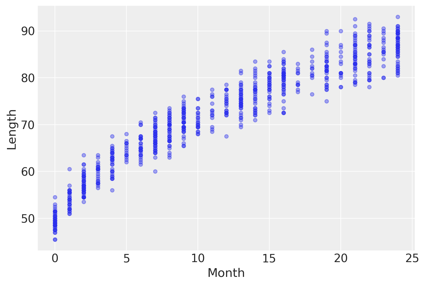
An example of such data is the lengths (heights) of newborn / toddler girls as a function of age (in months):
try:
    data = pd.read_csv("../data/babies.csv")
except FileNotFoundError:
    data = pd.read_csv(pm.get_data("babies.csv"))
data.plot.scatter("Month", "Length", alpha=0.4);
To model this data we are going to use this model:
with pm.Model(coords={"time_idx": np.arange(len(data))}) as model_babies:
    α = pm.Normal("α", sigma=10)
    β = pm.Normal("β", sigma=10)
    γ = pm.HalfNormal("γ", sigma=10)
    δ = pm.HalfNormal("δ", sigma=10)

    month = pm.Data("month", data.Month.values.astype(float), dims="time_idx")

    μ = pm.Deterministic("μ", α + β * month ** 0.5, dims="time_idx")
    ε = pm.Deterministic("ε", γ + δ * month, dims="time_idx")

    length = pm.Normal("length", mu=μ, sigma=ε, observed=data.Length, dims="time_idx")

    idata_babies = pm.sample(tune=2000, return_inferencedata=True)
Auto-assigning NUTS sampler...
Initializing NUTS using jitter+adapt_diag...
Multiprocess sampling (4 chains in 4 jobs)
NUTS: [δ, γ, β, α]
Sampling 4 chains for 2_000 tune and 1_000 draw iterations (8_000 + 4_000 draws total) took 23 seconds.
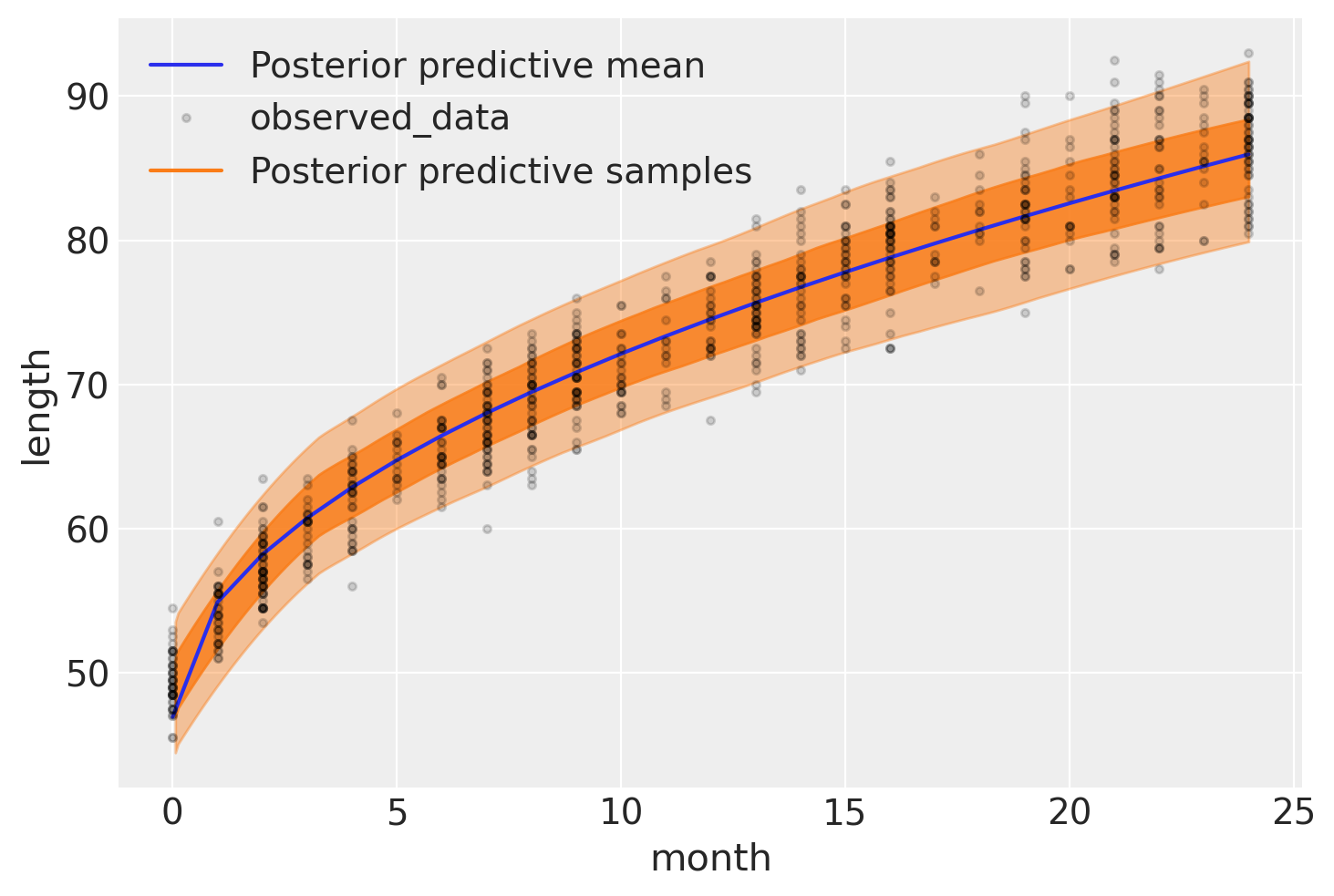
The following figure shows the result of our model. The expected length, \(\mu\), is represented with a blue curve, and two semi-transparent orange bands represent the 60% and 94% highest posterior density intervals of posterior predictive length measurements:
with model_babies:
    idata_babies.extend(
        az.from_pymc3(posterior_predictive=pm.sample_posterior_predictive(idata_babies))
    )
ax = az.plot_hdi(
    data.Month,
    idata_babies.posterior_predictive["length"],
    hdi_prob=0.6,
    fill_kwargs={"alpha": 0.8},
)
ax.plot(
    data.Month,
    idata_babies.posterior["μ"].mean(("chain", "draw")),
    label="Posterior predictive mean",
)
ax = az.plot_lm(
    idata=idata_babies,
    y="length",
    x="month",
    kind_pp="hdi",
    y_kwargs={"color": "k", "ms": 6, "alpha": 0.15},
    y_hat_fill_kwargs=dict(fill_kwargs={"alpha": 0.4}),
    axes=ax,
)
/home/oriol/miniconda3/envs/pymc-v3/lib/python3.9/site-packages/numpy/lib/shape_base.py:1250: VisibleDeprecationWarning: Creating an ndarray from ragged nested sequences (which is a list-or-tuple of lists-or-tuples-or ndarrays with different lengths or shapes) is deprecated. If you meant to do this, you must specify 'dtype=object' when creating the ndarray.
  c = _nx.array(A, copy=False, subok=True, ndmin=d)
At the moment of writing Osvaldo’s daughter is two weeks (\(\approx 0.5\) months) old, and thus he wonders how her length compares to the growth chart we have just created. One way to answer this question is to ask the model for the distribution of the variable length for babies of 0.5 months. Using PyMC3 we can ask this questions with the function sample_posterior_predictive , as this will return samples of Length conditioned on the obseved data and the estimated distribution of parameters, that is including uncertainties.
The only problem is that by default this function will return predictions for Length for the observed values of Month, and \(0.5\) months (the value Osvaldo cares about) has not been observed, – all measures are reported for integer months. The easier way to get predictions for non-observed values of Month is to pass new values to the Data container we defined above in our model. To do that, we need to use pm.set_data and then we just have to sample from the posterior predictve distribution:
ages_to_check = [0.5, 0.75]
with model_babies:
    pm.set_data({"month": ages_to_check})
    # we use two values instead of only 0.5 months to avoid triggering
    # https://github.com/pymc-devs/pymc3/issues/3640
    predictions = pm.sample_posterior_predictive(idata_babies)

    # add the generation predictions also to the inferencedata object
    # this is not necessary but allows for example storing data, posterior and predictions in the same file
    az.from_pymc3_predictions(
        predictions,
        idata_orig=idata_babies,
        inplace=True,
        # we update the dimensions and coordinates, we no longer have use for "time_idx"
        # as unique id. We'll now use the age in months as coordinate for better labeling and indexing
        # We duplicate the constant_data as coords though
        coords={"age (months)": ages_to_check},
        dims={"length": ["age (months)"], "month": ["age (months)"]},
    )
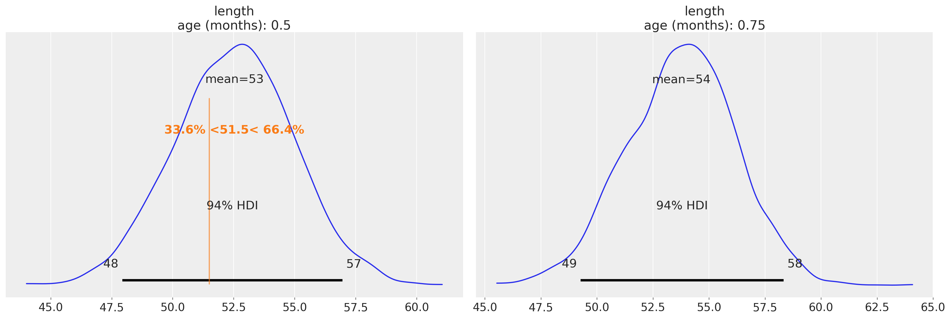
Now we can plot the expected distribution of lengths for 2-week old babies and compute additional quantities – for example the percentile of a child given her length. Here, let’s imagine that the child we’re interested in has a length of 51.5:
ref_length = 51.5

az.plot_posterior(
    idata_babies,
    group="predictions",
    ref_val={"length": [{"age (months)": 0.5, "ref_val": ref_length}]},
    labeller=az.labels.DimCoordLabeller(),
);
References
- 1
Osvaldo Martin. Bayesian analysis with Python: introduction to statistical modeling and probabilistic programming using PyMC3 and ArviZ. Packt Publishing Ltd, 2018.
Watermark
%load_ext watermark
%watermark -n -u -v -iv -w -p theano,xarray
Last updated: Sun Dec 19 2021

Python implementation: CPython
Python version       : 3.9.7
IPython version      : 7.29.0

theano: 1.1.2
xarray: 0.20.1

pandas    : 1.3.4
arviz     : 0.11.4
pymc3     : 3.11.4
matplotlib: 3.4.3
numpy     : 1.21.4

Watermark: 2.2.0
License notice
All the notebooks in this example gallery are provided under the MIT License which allows modification, and redistribution for any use provided the copyright and license notices are preserved.
Citing PyMC examples
To cite this notebook, use the DOI provided by Zenodo for the pymc-examples repository.
Important
Many notebooks are adapted from other sources: blogs, books… In such cases you should cite the original source as well.
Also remember to cite the relevant libraries used by your code.
Here is an citation template in bibtex:
@incollection{citekey,
  author    = "<notebook authors, see above>"
  title     = "<notebook title>",
  editor    = "PyMC Team",
  booktitle = "PyMC examples",
  doi       = "10.5281/zenodo.5832070"
}
which once rendered could look like:
-
Juan Martin Loyola
,
Kavya Jaiswal
,
Oriol Abril
. "Using shared variables (
Datacontainer adaptation)". In: PyMC Examples. Ed. by PyMC Team. DOI: 10.5281/zenodo.5832070