Dirichlet mixtures of multinomials

This example notebook demonstrates the use of a Dirichlet mixture of multinomials (a.k.a Dirichlet-multinomial or DM) to model categorical count data. Models like this one are important in a variety of areas, including natural language processing, ecology, bioinformatics, and more.

The Dirichlet-multinomial can be understood as draws from a Multinomial distribution where each sample has a slightly different probability vector, which is itself drawn from a common Dirichlet distribution. This contrasts with the Multinomial distribution, which assumes that all observations arise from a single fixed probability vector. This enables the Dirichlet-multinomial to accommodate more variable (a.k.a, over-dispersed) count data than the Multinomial.

Other examples of over-dispersed count distributions are the Beta-binomial (which can be thought of as a special case of the DM) or the Negative binomial distributions.

The DM is also an example of marginalizing a mixture distribution over its latent parameters. This notebook will demonstrate the performance benefits that come from taking that approach.

import arviz as az
import matplotlib.pyplot as plt
import numpy as np
import pymc3 as pm
import scipy as sp
import scipy.stats
import seaborn as sns

print(f"Running on PyMC3 v{pm.__version__}")

Running on PyMC3 v3.11.4

%config InlineBackend.figure_format = 'retina'
RANDOM_SEED = 8927
rng = np.random.default_rng(RANDOM_SEED)
az.style.use("arviz-darkgrid")

Simulation data

Let us simulate some over-dispersed, categorical count data for this example.

Here we are simulating from the DM distribution itself, so it is perhaps tautological to fit that model, but rest assured that data like these really do appear in the counts of different:

1. words in text corpuses [Rasmus E. Madsen and et al., 2005],

2. types of RNA molecules in a cell [Nowicka and Robinson, 2016],

3. items purchased by shoppers [G. J. Goodhardt and Chatfield, 1984].

Here we will discuss a community ecology example, pretending that we have observed counts of \(k=5\) different tree species in \(n=10\) different forests.

Our simulation will produce a two-dimensional matrix of integers (counts) where each row, (zero-)indexed by \(i \in (0...n-1)\), is an observation (different forest), and each column \(j \in (0...k-1)\) is a category (tree species). We’ll parameterize this distribution with three things:

• \(\mathrm{frac}\) : the expected fraction of each species, a \(k\)-dimensional vector on the simplex (i.e. sums-to-one)

• \(\mathrm{total\_count}\) : the total number of items tallied in each observation,

• \(\mathrm{conc}\) : the concentration, controlling the overdispersion of our data, where larger values result in our distribution more closely approximating the multinomial.

Here, and throughout this notebook, we’ve used a convenient reparameterization of the Dirichlet distribution from one to two parameters, \(\alpha=\mathrm{conc} \times \mathrm{frac}\), as this fits our desired interpretation.

Each observation from the DM is simulated by:

1. first obtaining a value on the \(k\)-simplex simulated as \(p_i \sim \mathrm{Dirichlet}(\alpha=\mathrm{conc} \times \mathrm{frac})\),

2. and then simulating \(\mathrm{counts}_i \sim \mathrm{Multinomial}(\mathrm{total\_count}, p_i)\).

Notice that each observation gets its own latent parameter \(p_i\), simulated independently from a common Dirichlet distribution.

true_conc = 6.0
true_frac = np.array([0.45, 0.30, 0.15, 0.09, 0.01])
trees = ["pine", "oak", "ebony", "rosewood", "mahogany"]  # Tree species observed
# fmt: off
forests = [  # Forests observed
    "sunderbans", "amazon", "arashiyama", "trossachs", "valdivian",
    "bosc de poblet", "font groga", "monteverde", "primorye", "daintree",
]
# fmt: on
k = len(trees)
n = len(forests)
total_count = 50

true_p = sp.stats.dirichlet(true_conc * true_frac).rvs(size=n)
observed_counts = np.vstack([sp.stats.multinomial(n=total_count, p=p_i).rvs() for p_i in true_p])

observed_counts

array([[34, 12,  0,  4,  0],
       [17, 24,  4,  5,  0],
       [38,  7,  1,  4,  0],
       [21,  8, 13,  8,  0],
       [32, 10,  6,  2,  0],
       [34,  8,  5,  3,  0],
       [33,  5, 11,  1,  0],
       [30,  8,  1, 11,  0],
       [18, 19,  8,  5,  0],
       [14, 25,  2,  9,  0]])

Multinomial model

The first model that we will fit to these data is a plain multinomial model, where the only parameter is the expected fraction of each category, \(\mathrm{frac}\), which we will give a Dirichlet prior. While the uniform prior (\(\alpha_j=1\) for each \(j\)) works well, if we have independent beliefs about the fraction of each tree, we could encode this into our prior, e.g. increasing the value of \(\alpha_j\) where we expect a higher fraction of species-\(j\).

coords = {"tree": trees, "forest": forests}
with pm.Model(coords=coords) as model_multinomial:
    frac = pm.Dirichlet("frac", a=np.ones(k), dims="tree")
    counts = pm.Multinomial(
        "counts", n=total_count, p=frac, observed=observed_counts, dims=("forest", "tree")
    )

pm.model_to_graphviz(model_multinomial)

Interestingly, NUTS frequently runs into numerical problems on this model, perhaps an example of the “Folk Theorem of Statistical Computing”.

Because of a couple of identities of the multinomial distribution, we could reparameterize this model in a number of ways—we would obtain equivalent models by exploding our \(n\) observations of \(\mathrm{total\_count}\) items into \((n \times \mathrm{total\_count})\) independent categorical trials, or collapsing them down into one Multinomial draw with \((n \times \mathrm{total\_count})\) items. (Importantly, this is not true for the DM distribution.)

Rather than actually fixing our problem through reparameterization, here we’ll instead switch to the Metropolis step method, which ignores some of the geometric pathologies of our naïve model.

Important: switching to Metropolis does not not fix our model’s issues, rather it sweeps them under the rug. In fact, if you try running this model with NUTS (PyMC3’s default step method), it will break loudly during sampling. When that happens, this should be a red alert that there is something wrong in our model.

You’ll also notice below that we have to increase considerably the number of draws we take from the posterior; this is because Metropolis is much less efficient at exploring the posterior than NUTS.

with model_multinomial:
    trace_multinomial = pm.sample(
        draws=5000, chains=4, step=pm.Metropolis(), return_inferencedata=True
    )

Multiprocess sampling (4 chains in 4 jobs)
Metropolis: [frac]

100.00% [24000/24000 00:04<00:00 Sampling 4 chains, 0 divergences]

Sampling 4 chains for 1_000 tune and 5_000 draw iterations (4_000 + 20_000 draws total) took 4 seconds.
The estimated number of effective samples is smaller than 200 for some parameters.

Let’s ignore the warning about inefficient sampling for now.

az.plot_trace(data=trace_multinomial, var_names=["frac"]);

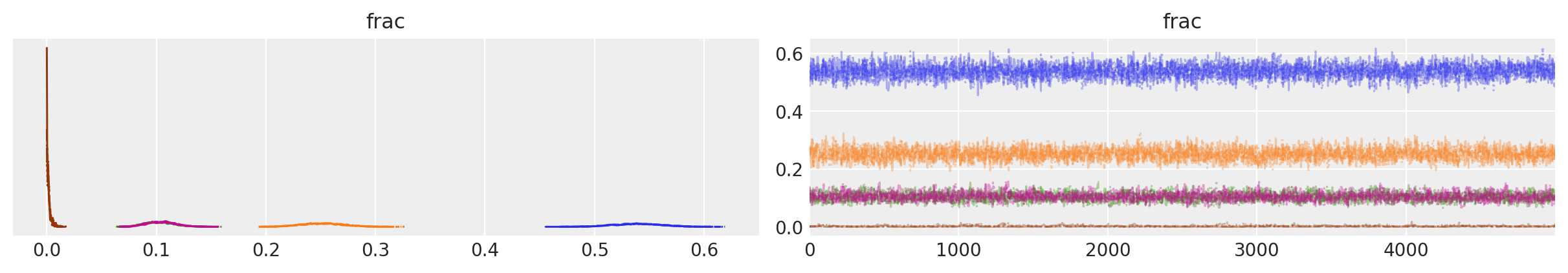
The trace plots look fairly good; visually, each parameter appears to be moving around the posterior well, although some sharp parts of the KDE plot suggests that sampling sometimes gets stuck in one place for a few steps.

summary_multinomial = az.summary(trace_multinomial, var_names=["frac"])

summary_multinomial = summary_multinomial.assign(
    ess_bulk_per_sec=lambda x: x.ess_bulk / trace_multinomial.posterior.sampling_time,
)

summary_multinomial

	mean	sd	hdi_3%	hdi_97%	mcse_mean	mcse_sd	ess_bulk	ess_tail	r_hat	ess_bulk_per_sec
frac[pine]	0.539	0.022	0.498	0.581	0.0	0.0	2451.0	3130.0	1.00	566.099382
frac[oak]	0.252	0.019	0.216	0.288	0.0	0.0	2005.0	3037.0	1.00	463.088234
frac[ebony]	0.103	0.014	0.079	0.130	0.0	0.0	1398.0	2090.0	1.00	322.891447
frac[rosewood]	0.104	0.013	0.079	0.129	0.0	0.0	1521.0	2082.0	1.00	351.300351
frac[mahogany]	0.002	0.002	0.000	0.005	0.0	0.0	122.0	119.0	1.02	28.177937

Likewise, diagnostics in the parameter summary table all look fine. Here I’ve added a column estimating the effective sample size per second of sampling.

Nonetheless, the fact that we were unable to use NUTS is still a red flag, and we should be very cautious in using these results.

az.plot_forest(trace_multinomial, var_names=["frac"])
for j, (y_tick, frac_j) in enumerate(zip(plt.gca().get_yticks(), reversed(true_frac))):
    plt.vlines(frac_j, ymin=y_tick - 0.45, ymax=y_tick + 0.45, color="black", linestyle="--")

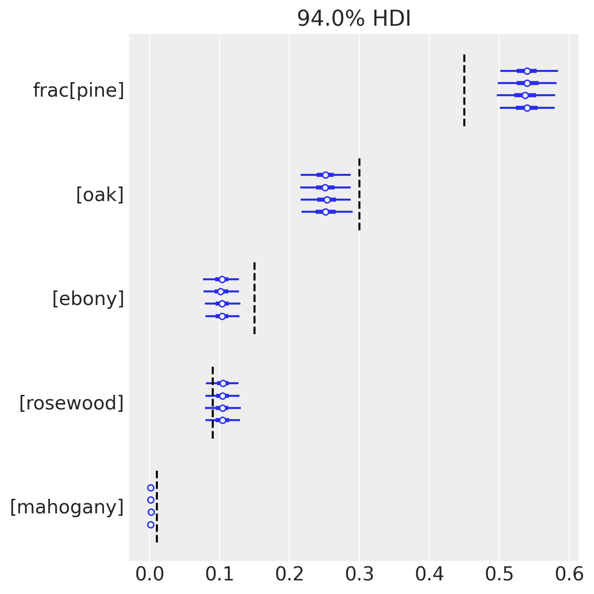
Here we’ve drawn a forest-plot, showing the mean and 94% HDIs from our posterior approximation. Interestingly, because we know what the underlying frequencies are for each species (dashed lines), we can comment on the accuracy of our inferences. And now the issues with our model become apparent; notice that the 94% HDIs don’t include the true values for tree species 0, 2, 3. We might have seen one HDI miss, but three???

…what’s going on?

Let’s troubleshoot this model using a posterior-predictive check, comparing our data to simulated data conditioned on our posterior estimates.

with model_multinomial:
    pp_samples = az.from_pymc3(
        posterior_predictive=pm.fast_sample_posterior_predictive(trace=trace_multinomial)
    )

# Concatenate with InferenceData object
trace_multinomial.extend(pp_samples)

cmap = plt.get_cmap("tab10")

fig, axs = plt.subplots(k, 1, sharex=True, sharey=True, figsize=(6, 8))
for j, ax in enumerate(axs):
    c = cmap(j)
    ax.hist(
        trace_multinomial.posterior_predictive.counts.sel(tree=trees[j]).values.flatten(),
        bins=np.arange(total_count),
        histtype="step",
        color=c,
        density=True,
        label="Post.Pred.",
    )
    ax.hist(
        (trace_multinomial.observed_data.counts.sel(tree=trees[j]).values.flatten()),
        bins=np.arange(total_count),
        color=c,
        density=True,
        alpha=0.25,
        label="Observed",
    )
    ax.axvline(
        true_frac[j] * total_count,
        color=c,
        lw=1.0,
        alpha=0.45,
        label="True",
    )
    ax.annotate(
        f"{trees[j]}",
        xy=(0.96, 0.9),
        xycoords="axes fraction",
        ha="right",
        va="top",
        color=c,
    )

axs[-1].legend(loc="upper center", fontsize=10)
axs[-1].set_xlabel("Count")
axs[-1].set_yticks([0, 0.5, 1.0])
axs[-1].set_ylim(0, 0.6);

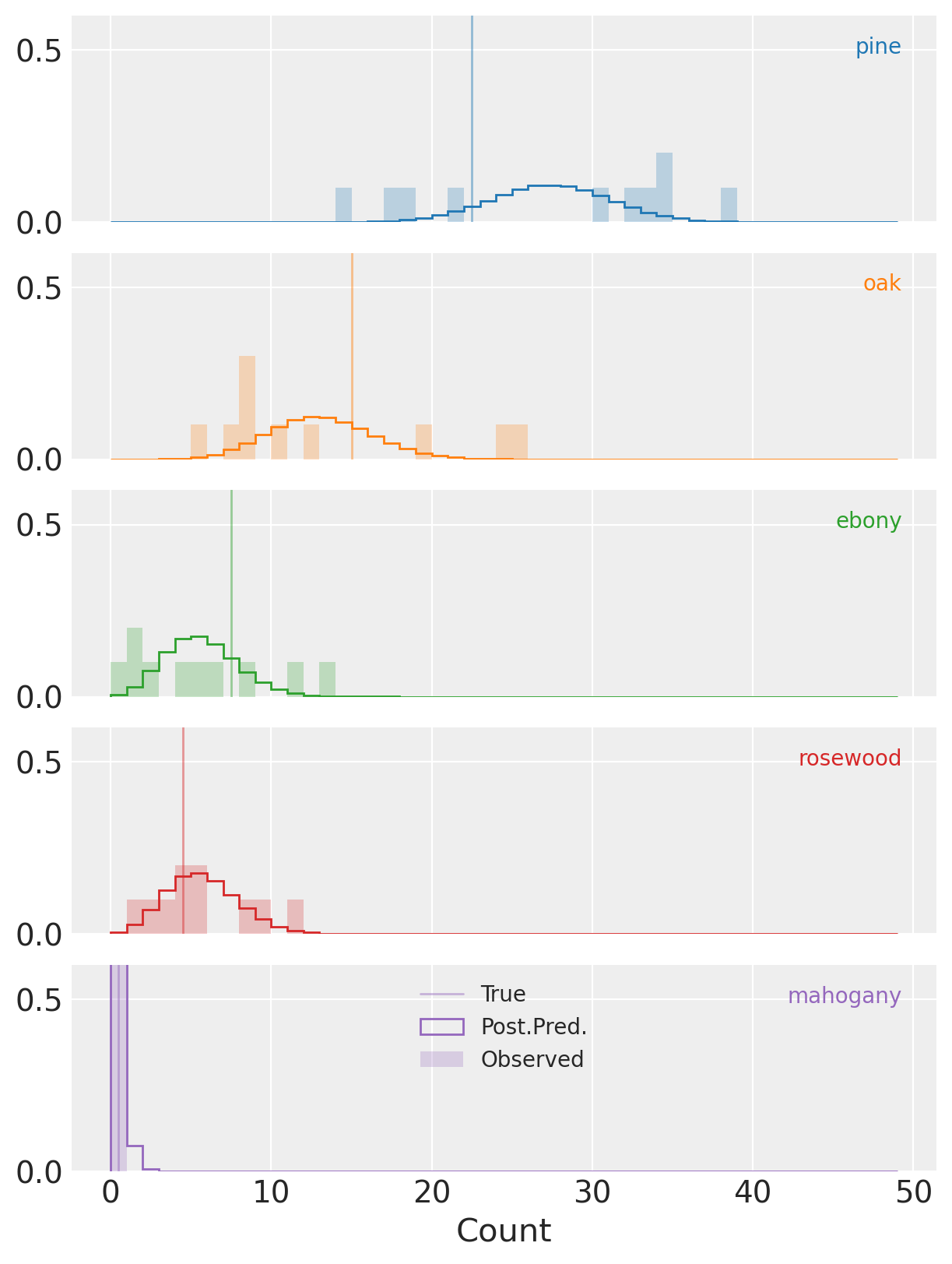
Here we’re plotting histograms of the predicted counts against the observed counts for each species.

(Notice that the y-axis isn’t full height and clips the distributions for species-4 in purple.)

And now we can start to see why our posterior HDI deviates from the true parameters for three of five species (vertical lines). See that for all of the species the observed counts are frequently quite far from the predictions conditioned on the posterior distribution. This is particularly obvious for (e.g.) species-2 where we have one observation of more than 20 trees of this species, despite the posterior predicitive mass being concentrated far below that.

This is overdispersion at work, and a clear sign that we need to adjust our model to accomodate it.

Posterior predictive checks are one of the best ways to diagnose model misspecification, and this example is no different.

Dirichlet-Multinomial Model - Explicit Mixture

Let’s go ahead and model our data using the DM distribution.

For this model we’ll keep the same prior on the expected frequencies of each species, \(\mathrm{frac}\). We’ll also add a strictly positive parameter, \(\mathrm{conc}\), for the concentration.

In this iteration of our model we’ll explicitly include the latent multinomial probability, \(p_i\), modeling the \(\mathrm{true\_p}_i\) from our simulations (which we would not observe in the real world).

with pm.Model(coords=coords) as model_dm_explicit:
    frac = pm.Dirichlet("frac", a=np.ones(k), dims="tree")
    conc = pm.Lognormal("conc", mu=1, sigma=1)
    p = pm.Dirichlet("p", a=frac * conc, dims=("forest", "tree"))
    counts = pm.Multinomial(
        "counts", n=total_count, p=p, observed=observed_counts, dims=("forest", "tree")
    )

pm.model_to_graphviz(model_dm_explicit)

Compare this diagram to the first. Here the latent, Dirichlet distributed \(p\) separates the multinomial from the expected frequencies, \(\mathrm{frac}\), accounting for overdispersion of counts relative to the simple multinomial model.

with model_dm_explicit:
    trace_dm_explicit = pm.sample(chains=4, return_inferencedata=True)

Auto-assigning NUTS sampler...
Initializing NUTS using jitter+adapt_diag...
Multiprocess sampling (4 chains in 4 jobs)
NUTS: [p, conc, frac]

100.00% [8000/8000 03:12<00:00 Sampling 4 chains, 42 divergences]

Sampling 4 chains for 1_000 tune and 1_000 draw iterations (4_000 + 4_000 draws total) took 193 seconds.
There were 3 divergences after tuning. Increase `target_accept` or reparameterize.
There were 8 divergences after tuning. Increase `target_accept` or reparameterize.
There were 13 divergences after tuning. Increase `target_accept` or reparameterize.
The acceptance probability does not match the target. It is 0.6608964239952206, but should be close to 0.8. Try to increase the number of tuning steps.
There were 18 divergences after tuning. Increase `target_accept` or reparameterize.
The acceptance probability does not match the target. It is 0.8823566155656549, but should be close to 0.8. Try to increase the number of tuning steps.
The rhat statistic is larger than 1.05 for some parameters. This indicates slight problems during sampling.
The estimated number of effective samples is smaller than 200 for some parameters.

We got a warning, although we’ll ignore it for now. More interesting is how much longer it took to sample this model than the first. This may be because our model has an additional ~\((n \times k)\) parameters, but it seems like there are other geometric challenges for NUTS as well.

We’ll see if we can fix these in the next model, but for now let’s take a look at the traces.

az.plot_trace(data=trace_dm_explicit, var_names=["frac", "conc"]);

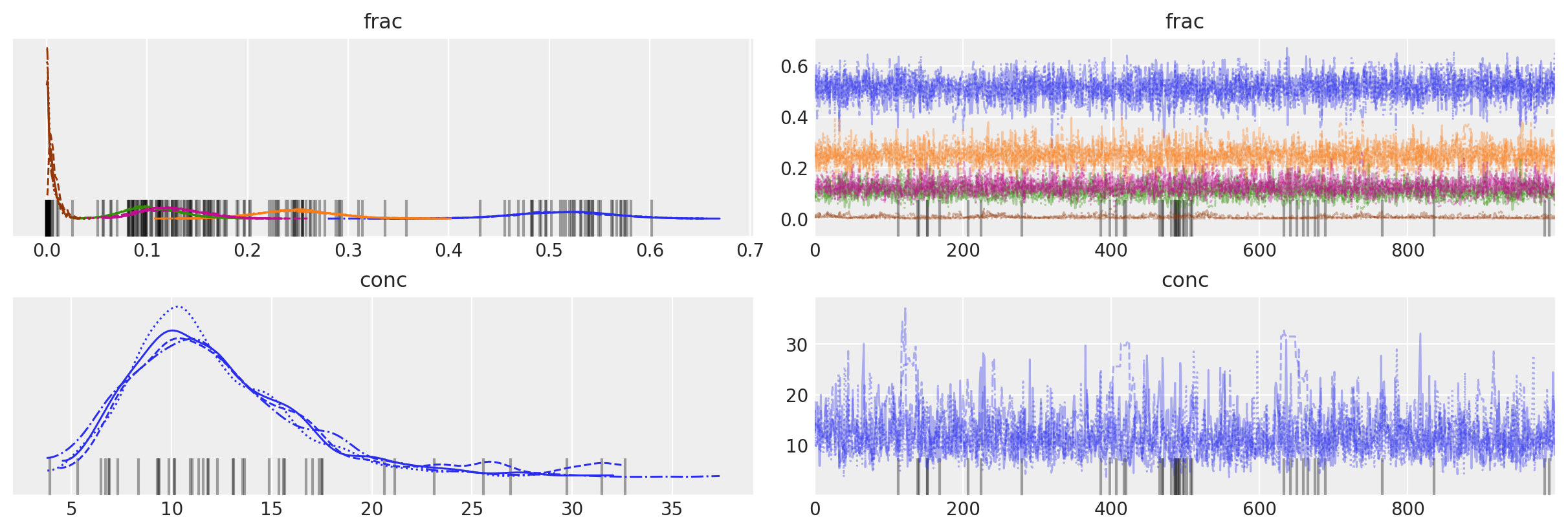
Obviously some sampling issues, but it’s hard to see where divergences are occurring.

az.plot_forest(trace_dm_explicit, var_names=["frac"])
for j, (y_tick, frac_j) in enumerate(zip(plt.gca().get_yticks(), reversed(true_frac))):
    plt.vlines(frac_j, ymin=y_tick - 0.45, ymax=y_tick + 0.45, color="black", linestyle="--")

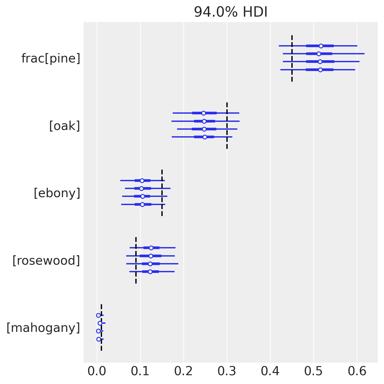
On the other hand, since we know the ground-truth for \(\mathrm{frac}\), we can congratulate ourselves that the HDIs include the true values for all of our species!

Modeling this mixture has made our inferences robust to the overdispersion of counts, while the plain multinomial is very sensitive. Notice that the HDI is much wider than before for each \(\mathrm{frac}_i\). In this case that makes the difference between correct and incorrect inferences.

summary_dm_explicit = az.summary(trace_dm_explicit, var_names=["frac", "conc"])
summary_dm_explicit = summary_dm_explicit.assign(
    ess_bulk_per_sec=lambda x: x.ess_bulk / trace_dm_explicit.posterior.sampling_time,
)

summary_dm_explicit

	mean	sd	hdi_3%	hdi_97%	mcse_mean	mcse_sd	ess_bulk	ess_tail	r_hat	ess_bulk_per_sec
frac[pine]	0.514	0.048	0.429	0.611	0.001	0.001	2170.0	2441.0	1.00	11.268102
frac[oak]	0.248	0.040	0.175	0.325	0.001	0.001	2169.0	1995.0	1.00	11.262909
frac[ebony]	0.106	0.028	0.056	0.161	0.001	0.001	1241.0	1403.0	1.00	6.444108
frac[rosewood]	0.126	0.031	0.069	0.181	0.001	0.001	889.0	380.0	1.01	4.616287
frac[mahogany]	0.006	0.006	0.000	0.016	0.001	0.000	51.0	162.0	1.07	0.264826
conc	12.348	4.642	4.532	20.406	0.254	0.199	485.0	324.0	1.01	2.518447

This is great, but we can do better. The larger \(\hat{R}\) value for \(\mathrm{frac}_4\) is mildly concerning, and it’s surprising that our \(\mathrm{ESS} \; \mathrm{sec}^{-1}\) is relatively small.

Dirichlet-Multinomial Model - Marginalized

Happily, the Dirichlet distribution is conjugate to the multinomial and therefore there’s a convenient, closed-form for the marginalized distribution, i.e. the Dirichlet-multinomial distribution, which was added to PyMC3 in 3.11.0.

Let’s take advantage of this, marginalizing out the explicit latent parameter, \(p_i\), replacing the combination of this node and the multinomial with the DM to make an equivalent model.

with pm.Model(coords=coords) as model_dm_marginalized:
    frac = pm.Dirichlet("frac", a=np.ones(k), dims="tree")
    conc = pm.Lognormal("conc", mu=1, sigma=1)
    counts = pm.DirichletMultinomial(
        "counts", n=total_count, a=frac * conc, observed=observed_counts, dims=("forest", "tree")
    )

pm.model_to_graphviz(model_dm_marginalized)

The plate diagram shows that we’ve collapsed what had been the latent Dirichlet and the multinomial nodes together into a single DM node.

with model_dm_marginalized:
    trace_dm_marginalized = pm.sample(chains=4, return_inferencedata=True)

Auto-assigning NUTS sampler...
Initializing NUTS using jitter+adapt_diag...
Multiprocess sampling (4 chains in 4 jobs)
NUTS: [conc, frac]

100.00% [8000/8000 00:06<00:00 Sampling 4 chains, 0 divergences]

Sampling 4 chains for 1_000 tune and 1_000 draw iterations (4_000 + 4_000 draws total) took 7 seconds.

It samples much more quickly and without any of the warnings from before!

az.plot_trace(data=trace_dm_marginalized, var_names=["frac", "conc"]);

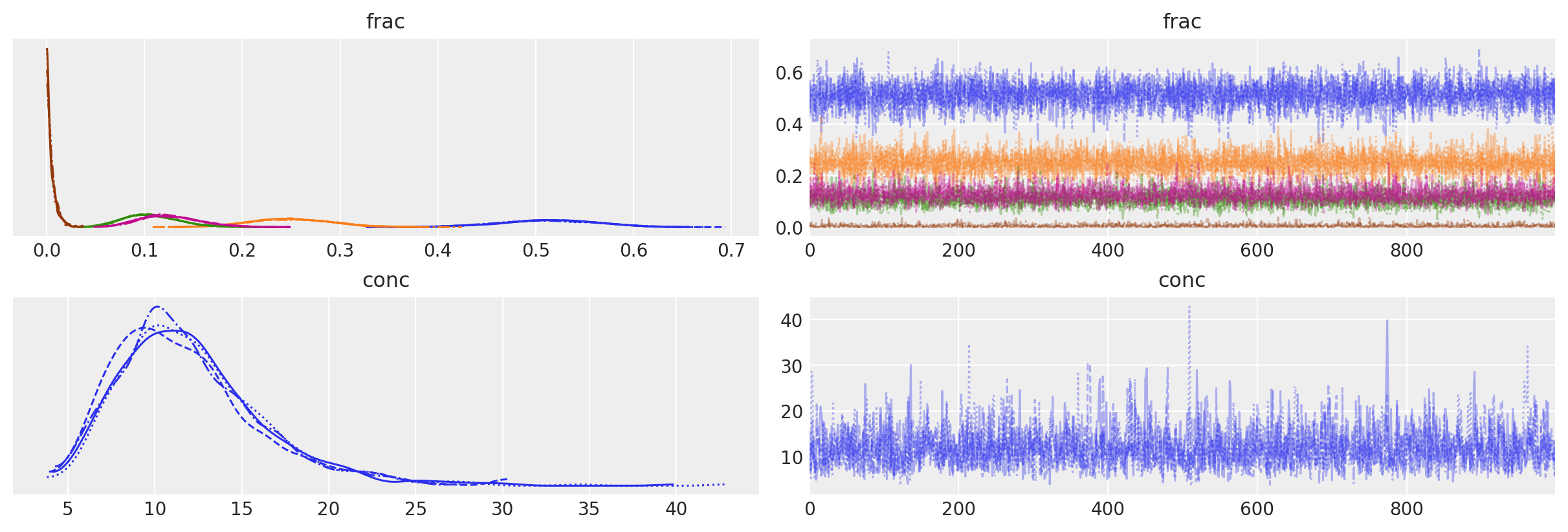
Trace plots look fuzzy and KDEs are clean.

summary_dm_marginalized = az.summary(trace_dm_marginalized, var_names=["frac", "conc"])
summary_dm_marginalized = summary_dm_marginalized.assign(
    ess_mean_per_sec=lambda x: x.ess_bulk / trace_dm_marginalized.posterior.sampling_time,
)
assert all(summary_dm_marginalized.r_hat < 1.03)

summary_dm_marginalized

	mean	sd	hdi_3%	hdi_97%	mcse_mean	mcse_sd	ess_bulk	ess_tail	r_hat	ess_mean_per_sec
frac[pine]	0.512	0.050	0.418	0.605	0.001	0.000	5269.0	3185.0	1.0	754.444438
frac[oak]	0.249	0.042	0.168	0.322	0.001	0.000	6084.0	3613.0	1.0	871.140627
frac[ebony]	0.107	0.028	0.059	0.162	0.000	0.000	4129.0	2818.0	1.0	591.212960
frac[rosewood]	0.126	0.030	0.073	0.183	0.000	0.000	4540.0	3209.0	1.0	650.062203
frac[mahogany]	0.005	0.005	0.000	0.015	0.000	0.000	1143.0	964.0	1.0	163.661035
conc	11.984	4.188	4.883	19.291	0.085	0.062	2559.0	2554.0	1.0	366.411713

We see that \(\hat{R}\) is close to \(1\) everywhere and \(\mathrm{ESS} \; \mathrm{sec}^{-1}\) is much higher. Our reparameterization (marginalization) has greatly improved the sampling! (And, thankfully, the HDIs look similar to the other model.)

This all looks very good, but what if we didn’t have the ground-truth?

Posterior predictive checks to the rescue (again)!

with model_dm_marginalized:
    pp_samples = az.from_pymc3(
        posterior_predictive=pm.fast_sample_posterior_predictive(trace_dm_marginalized)
    )

# Concatenate with InferenceData object
trace_dm_marginalized.extend(pp_samples)

cmap = plt.get_cmap("tab10")

fig, axs = plt.subplots(k, 2, sharex=True, sharey=True, figsize=(8, 8))
for j, row in enumerate(axs):
    c = cmap(j)
    for _trace, ax in zip([trace_dm_marginalized, trace_multinomial], row):
        ax.hist(
            _trace.posterior_predictive.counts.sel(tree=trees[j]).values.flatten(),
            bins=np.arange(total_count),
            histtype="step",
            color=c,
            density=True,
            label="Post.Pred.",
        )
        ax.hist(
            (_trace.observed_data.counts.sel(tree=trees[j]).values.flatten()),
            bins=np.arange(total_count),
            color=c,
            density=True,
            alpha=0.25,
            label="Observed",
        )
        ax.axvline(
            true_frac[j] * total_count,
            color=c,
            lw=1.0,
            alpha=0.45,
            label="True",
        )
    row[1].annotate(
        f"{trees[j]}",
        xy=(0.96, 0.9),
        xycoords="axes fraction",
        ha="right",
        va="top",
        color=c,
    )

axs[-1, -1].legend(loc="upper center", fontsize=10)
axs[0, 1].set_title("Multinomial")
axs[0, 0].set_title("Dirichlet-multinomial")
axs[-1, 0].set_xlabel("Count")
axs[-1, 1].set_xlabel("Count")
axs[-1, 0].set_yticks([0, 0.5, 1.0])
axs[-1, 0].set_ylim(0, 0.6)
ax.set_ylim(0, 0.6);

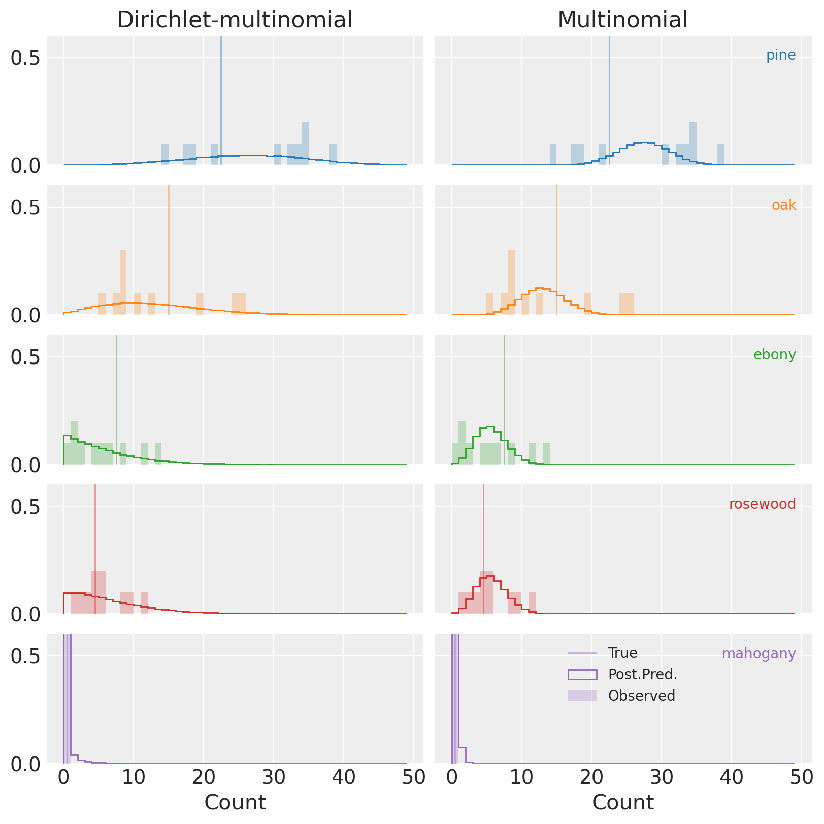
(Notice, again, that the y-axis isn’t full height, and clips the distributions for species-4 in purple.)

Compared to the multinomial (plots on the right), PPCs for the DM (left) show that the observed data is an entirely reasonable realization of our model. This is great news!

Model Comparison

Let’s go a step further and try to put a number on how much better our DM model is relative to the raw multinomial. We’ll use leave-one-out cross validation to compare the out-of-sample predictive ability of the two.

az.compare(
    {"multinomial": trace_multinomial, "dirichlet_multinomial": trace_dm_marginalized}, ic="loo"
)

	rank	loo	p_loo	d_loo	weight	se	dse	warning	loo_scale
dirichlet_multinomial	0	-90.100582	2.888430	0.000000	1.0	2.307516	0.000000	False	log
multinomial	1	-117.149775	11.637356	27.049193	0.0	9.122851	7.459096	False	log

Unsurprisingly, the DM outclasses the multinomial by a mile, assigning a weight of nearly 100% to the over-dispersed model. We can conclude that between the two, the DM should be greatly favored for prediction, parameter inference, etc.

Conclusions

Obviously the DM is not a perfect model in every case, but it is often a better choice than the multinomial, much more robust while taking on just one additional parameter.

There are a number of shortcomings to the DM that we should keep in mind when selecting a model. The biggest problem is that, while more flexible than the multinomial, the DM still ignores the possibility of underlying correlations between categories. If one of our tree species relies on another, for instance, the model we’ve used here will not effectively account for this. In that case, swapping the vanilla Dirichlet distribution for something fancier (e.g. the Generalized Dirichlet or Logistic-Multivariate Normal) may be worth considering.

References

1

Charles Elkan Rasmus E. Madsen, David Kauchak and et al. Modeling word burstiness using the dirichlet distribution. Aug 2005. URL: https://dl.acm.org/doi/10.1145/1102351.1102420.

2

Malgorzata Nowicka and Mark D. Robinson. Drimseq: a dirichlet-multinomial framework for multivariate count outcomes in genomics. Dec 2016. URL: https://f1000research.com/articles/5-1356/v2.

3

A. S. C. Ehrenberg G. J. Goodhardt and C. Chatfield. The dirichlet: a comprehensive model of buying behaviour. 1984. URL: https://www.jstor.org/stable/2981696.

Authors

• Authored by Byron J. Smith on Jan, 2021 (pymc-examples#18)

• Updated by Abhipsha Das and Oriol Abril-Pla on August, 2021 (pymc-examples#212)

Watermark

%load_ext watermark
%watermark -n -u -v -iv -w -p theano,xarray

Last updated: Sun Jan 09 2022

Python implementation: CPython
Python version       : 3.9.7
IPython version      : 7.29.0

theano: 1.1.2
xarray: 0.20.1

pymc3     : 3.11.4
arviz     : 0.11.4
numpy     : 1.21.4
matplotlib: 3.4.3
seaborn   : 0.11.2
scipy     : 1.7.2

Watermark: 2.2.0

• Byron J. Smith , Abhipsha Das , Oriol Abril-Pla . "Dirichlet mixtures of multinomials". In: PyMC Examples. Ed. by PyMC Team. DOI: 10.5281/zenodo.5832070