


A Primer on Bayesian Methods for Multilevel Modeling
Hierarchical or multilevel modeling is a generalization of regression modeling. Multilevel models are regression models in which the constituent model parameters are given probability models. This implies that model parameters are allowed to vary by group. Observational units are often naturally clustered. Clustering induces dependence between observations, despite random sampling of clusters and random sampling within clusters.
A hierarchical model is a particular multilevel model where parameters are nested within one another. Some multilevel structures are not hierarchical – e.g. “country” and “year” are not nested, but may represent separate, but overlapping, clusters of parameters. We will motivate this topic using an environmental epidemiology example.
Example: Radon contamination Gelman and Hill [2006]
Radon is a radioactive gas that enters homes through contact points with the ground. It is a carcinogen that is the primary cause of lung cancer in non-smokers. Radon levels vary greatly from household to household.
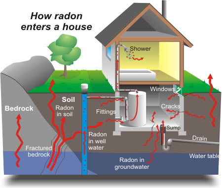
The EPA did a study of radon levels in 80,000 houses. There are two important predictors:
measurement in basement or first floor (radon higher in basements)
county uranium level (positive correlation with radon levels)
We will focus on modeling radon levels in Minnesota.
The hierarchy in this example is households within county.
Data organization
First, we import the data from a local file, and extract Minnesota’s data.
import os

import arviz as az
import matplotlib.pyplot as plt
import numpy as np
import pandas as pd
import pymc3 as pm
import xarray as xr

from theano import tensor as tt

print(f"Running on PyMC3 v{pm.__version__}")
Running on PyMC3 v3.11.4
RANDOM_SEED = 8924
az.style.use("arviz-darkgrid")
# Import radon data
try:
    srrs2 = pd.read_csv(os.path.join("..", "data", "srrs2.dat"))
except FileNotFoundError:
    srrs2 = pd.read_csv(pm.get_data("srrs2.dat"))

srrs2.columns = srrs2.columns.map(str.strip)
srrs_mn = srrs2[srrs2.state == "MN"].copy()
Next, obtain the county-level predictor, uranium, by combining two variables.
srrs_mn["fips"] = srrs_mn.stfips * 1000 + srrs_mn.cntyfips
cty = pd.read_csv(pm.get_data("cty.dat"))
cty_mn = cty[cty.st == "MN"].copy()
cty_mn["fips"] = 1000 * cty_mn.stfips + cty_mn.ctfips
Use the merge method to combine home- and county-level information in a single DataFrame.
srrs_mn = srrs_mn.merge(cty_mn[["fips", "Uppm"]], on="fips")
srrs_mn = srrs_mn.drop_duplicates(subset="idnum")
u = np.log(srrs_mn.Uppm).unique()

n = len(srrs_mn)
srrs_mn.head()
| idnum | state | state2 | stfips | zip | region | typebldg | floor | room | basement | ... | stopdt | activity | pcterr | adjwt | dupflag | zipflag | cntyfips | county | fips | Uppm | |
|---|---|---|---|---|---|---|---|---|---|---|---|---|---|---|---|---|---|---|---|---|---|
| 0 | 5081 | MN | MN | 27 | 55735 | 5 | 1 | 1 | 3 | N | ... | 12288 | 2.2 | 9.7 | 1146.499190 | 1 | 0 | 1 | AITKIN | 27001 | 0.502054 |
| 1 | 5082 | MN | MN | 27 | 55748 | 5 | 1 | 0 | 4 | Y | ... | 12088 | 2.2 | 14.5 | 471.366223 | 0 | 0 | 1 | AITKIN | 27001 | 0.502054 |
| 2 | 5083 | MN | MN | 27 | 55748 | 5 | 1 | 0 | 4 | Y | ... | 21188 | 2.9 | 9.6 | 433.316718 | 0 | 0 | 1 | AITKIN | 27001 | 0.502054 |
| 3 | 5084 | MN | MN | 27 | 56469 | 5 | 1 | 0 | 4 | Y | ... | 123187 | 1.0 | 24.3 | 461.623670 | 0 | 0 | 1 | AITKIN | 27001 | 0.502054 |
| 4 | 5085 | MN | MN | 27 | 55011 | 3 | 1 | 0 | 4 | Y | ... | 13088 | 3.1 | 13.8 | 433.316718 | 0 | 0 | 3 | ANOKA | 27003 | 0.428565 |
5 rows × 27 columns
We also need a lookup table (dict) for each unique county, for indexing.
srrs_mn.county = srrs_mn.county.map(str.strip)
mn_counties = srrs_mn.county.unique()
counties = len(mn_counties)
county_lookup = dict(zip(mn_counties, range(counties)))
Finally, create local copies of variables.
county = srrs_mn["county_code"] = srrs_mn.county.replace(county_lookup).values
radon = srrs_mn.activity
srrs_mn["log_radon"] = log_radon = np.log(radon + 0.1).values
floor = srrs_mn.floor.values
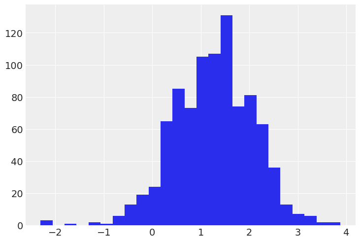
Distribution of radon levels in MN (log scale):
srrs_mn.log_radon.hist(bins=25);
Conventional approaches
The two conventional alternatives to modeling radon exposure represent the two extremes of the bias-variance tradeoff:
Complete pooling:
Treat all counties the same, and estimate a single radon level.
No pooling:
Model radon in each county independently.
where \(j = 1,\ldots,85\)
The errors \(\epsilon_i\) may represent measurement error, temporal within-house variation, or variation among houses.
We’ll start by estimating the slope and intercept for the complete pooling model. You’ll notice that we used an index variable instead of an indicator variable in the linear model below. There are two main reasons. One, this generalizes well to more-than-two-category cases. Two, this approach correctly considers that neither category has more prior uncertainty than the other. On the contrary, the indicator variable approach necessarily assumes that one of the categories has more uncertainty than the other: here, the cases when floor=1 would take into account 2 priors (\(\alpha + \beta\)), whereas cases when floor=0 would have only one prior (\(\alpha\)). But a priori we aren’t more unsure about floor measurements than about basement measurements, so it makes sense to give them the same prior uncertainty.
Now for the model:
coords = {"Level": ["Basement", "Floor"], "obs_id": np.arange(floor.size)}
with pm.Model(coords=coords) as pooled_model:
    floor_idx = pm.Data("floor_idx", floor, dims="obs_id")
    a = pm.Normal("a", 0.0, sigma=10.0, dims="Level")

    theta = a[floor_idx]
    sigma = pm.Exponential("sigma", 1.0)

    y = pm.Normal("y", theta, sigma=sigma, observed=log_radon, dims="obs_id")

pm.model_to_graphviz(pooled_model)

You may be wondering why we are using the pm.Data container above even though the variable floor_idx is not an observed variable nor a parameter of the model. As you’ll see, this will make our lives much easier when we’ll plot and diagnose our model. In short, this will tell ArviZ that floor_idx is information used by the model to index variables. ArviZ will thus include floor_idx as a variable in the constant_data group of the resulting InferenceData object. Moreover, including floor_idx in the InferenceData object makes sharing and reproducing analysis much easier, all the data needed to analyze or rerun the model is stored there.
Before running the model let’s do some prior predictive checks. Indeed, having sensible priors is not only a way to incorporate scientific knowledge into the model, it can also help and make the MCMC machinery faster – here we are dealing with a simple linear regression, so no link function comes and distorts the outcome space; but one day this will happen to you and you’ll need to think hard about your priors to help your MCMC sampler. So, better to train ourselves when it’s quite easy than having to learn when it’s very hard… There is a really neat function to do that in PyMC3:
with pooled_model:
    prior_checks = pm.sample_prior_predictive(random_seed=RANDOM_SEED)
    idata_prior = az.from_pymc3(prior=prior_checks)

_, ax = plt.subplots()
idata_prior.prior.plot.scatter(x="Level", y="a", color="k", alpha=0.2, ax=ax)
ax.set_ylabel("Mean log radon level");
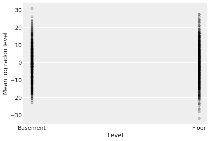
ArviZ InferenceData uses xarray.Datasets under the hood, which give access to several common plotting functions with .plot. In this case, we want scatter plot of the mean log radon level (which is stored in variable a) for each of the two levels we are considering. If our desired plot is supported by xarray plotting capabilities, we can take advantage of xarray to automatically generate both plot and labels for us. Notice how everything is directly plotted and annotated, the only change we need to do is renaming the y axis label from a to Mean log radon level.
I’m no expert in radon levels, but, before seing the data, these priors seem to allow for quite a wide range of the mean log radon level. But don’t worry, we can always change these priors if sampling gives us hints that they might not be appropriate – after all, priors are assumptions, not oaths; and as most assumptions, they can be tested.
However, we can already think of an improvement. Do you see it? Remember what we said at the beginning: radon levels tend to be higher in basements, so we could incorporate this prior scientific knowledge into our model by giving \(a_{basement}\) a higher mean than \(a_{floor}\). Here, there are so much data that the prior should be washed out anyway, but we should keep this fact in mind – for future cases or if sampling proves more difficult than expected…
Speaking of sampling, let’s fire up the Bayesian machinery!
with pooled_model:
    pooled_trace = pm.sample(random_seed=RANDOM_SEED, return_inferencedata=False)
    pooled_idata = az.from_pymc3(pooled_trace)
az.summary(pooled_idata, round_to=2)
Auto-assigning NUTS sampler...
Initializing NUTS using jitter+adapt_diag...
Multiprocess sampling (4 chains in 4 jobs)
NUTS: [sigma, a]
Sampling 4 chains for 1_000 tune and 1_000 draw iterations (4_000 + 4_000 draws total) took 17 seconds.
| mean | sd | hdi_3% | hdi_97% | mcse_mean | mcse_sd | ess_bulk | ess_tail | r_hat | |
|---|---|---|---|---|---|---|---|---|---|
| a[Basement] | 1.36 | 0.03 | 1.31 | 1.42 | 0.0 | 0.0 | 4939.09 | 2973.08 | 1.0 |
| a[Floor] | 0.78 | 0.06 | 0.64 | 0.88 | 0.0 | 0.0 | 5350.48 | 2815.15 | 1.0 |
| sigma | 0.79 | 0.02 | 0.76 | 0.83 | 0.0 | 0.0 | 5249.73 | 3172.00 | 1.0 |
No divergences and a sampling that only took seconds – this is the Flash of samplers! Here the chains look very good (good R hat, good effective sample size, small sd), but remember to check your chains after sampling – az.plot_trace is usually a good start.
Let’s see what it means on the outcome space: did the model pick-up the negative relationship between floor measurements and log radon levels? What’s the uncertainty around its estimates? To estimate the uncertainty around the household radon levels (not the average level, but measurements that would be likely in households), we need to sample the likelihood y from the model. In another words, we need to do posterior predictive checks:
with pooled_model:
    ppc = pm.sample_posterior_predictive(pooled_trace, random_seed=RANDOM_SEED)
    pooled_idata = az.from_pymc3(pooled_trace, posterior_predictive=ppc, prior=prior_checks)
We have now converted our trace and posterior predictive samples into an arviz.InferenceData object. InferenceData is specifically designed to centralize all the relevant quantities of a Bayesian inference workflow into a single object. This will also make the rendering of plots and diagnostics faster – otherwise ArviZ will need to convert your trace to InferenceData each time you call it.
pooled_idata
-
- chain: 4
- draw: 1000
- Level: 2
- chain(chain)int640 1 2 3
array([0, 1, 2, 3])
- draw(draw)int640 1 2 3 4 5 ... 995 996 997 998 999
array([ 0, 1, 2, ..., 997, 998, 999])
- Level(Level)<U8'Basement' 'Floor'
array(['Basement', 'Floor'], dtype='<U8')
- a(chain, draw, Level)float641.36 0.8198 1.379 ... 1.372 0.7468
array([[[1.36003089, 0.81977509], [1.37920405, 0.66650977], [1.38843718, 0.73977375], ..., [1.38086296, 0.77455862], [1.36854134, 0.76905776], [1.36623636, 0.8060241 ]], [[1.304446 , 0.78838489], [1.27732718, 0.7844349 ], [1.28471339, 0.79588536], ..., [1.33343979, 0.74229685], [1.377951 , 0.78555699], [1.40959545, 0.82210539]], [[1.37989301, 0.78526267], [1.35047441, 0.799208 ], [1.35047441, 0.799208 ], ..., [1.39349902, 0.72440342], [1.33797696, 0.71317817], [1.34251786, 0.73056496]], [[1.3738162 , 0.67495502], [1.37445448, 0.8296412 ], [1.35985069, 0.76263082], ..., [1.41241666, 0.79403558], [1.38569124, 0.76835064], [1.37203421, 0.74682483]]]) - sigma(chain, draw)float640.8159 0.7656 ... 0.7835 0.8056
array([[0.81591061, 0.76558984, 0.78261922, ..., 0.79732304, 0.79384231, 0.82277114], [0.79839322, 0.79900885, 0.78482389, ..., 0.75153775, 0.76896342, 0.79116258], [0.79324547, 0.78808448, 0.78808448, ..., 0.80481182, 0.81237951, 0.81429943], [0.81938454, 0.76473314, 0.81544394, ..., 0.78901935, 0.78354637, 0.80558638]])
- created_at :
- 2021-11-14T10:20:01.533738
- arviz_version :
- 0.11.4
- inference_library :
- pymc3
- inference_library_version :
- 3.11.4
- sampling_time :
- 16.85056209564209
- tuning_steps :
- 1000
<xarray.Dataset>
Dimensions:  (chain: 4, draw: 1000, Level: 2)
Coordinates:
  * chain    (chain) int64 0 1 2 3
  * draw     (draw) int64 0 1 2 3 4 5 6 7 8 ... 992 993 994 995 996 997 998 999
  * Level    (Level) <U8 'Basement' 'Floor'
Data variables:
    a        (chain, draw, Level) float64 1.36 0.8198 1.379 ... 1.372 0.7468
    sigma    (chain, draw) float64 0.8159 0.7656 0.7826 ... 0.789 0.7835 0.8056
Attributes:
    created_at:                 2021-11-14T10:20:01.533738
    arviz_version:              0.11.4
    inference_library:          pymc3
    inference_library_version:  3.11.4
    sampling_time:              16.85056209564209
    tuning_steps:               1000
xarray.Dataset -
- chain: 4
- draw: 1000
- obs_id: 919
- chain(chain)int640 1 2 3
array([0, 1, 2, 3])
- draw(draw)int640 1 2 3 4 5 ... 995 996 997 998 999
array([ 0, 1, 2, ..., 997, 998, 999])
- obs_id(obs_id)int640 1 2 3 4 5 ... 914 915 916 917 918
array([ 0, 1, 2, ..., 916, 917, 918])
- y(chain, draw, obs_id)float641.725 1.314 1.424 ... 2.057 2.273
array([[[ 1.72472548e+00, 1.31445158e+00, 1.42365617e+00, ..., 1.18250872e+00, 2.75272483e+00, 2.65149091e+00], [ 1.18964007e+00, 1.50385029e+00, 1.18541771e+00, ..., 2.11849713e+00, 3.80127359e-01, 1.91266834e+00], [ 8.51442991e-01, 1.33360977e+00, 1.20450890e+00, ..., 8.59996457e-01, 1.15073916e+00, 2.03686860e+00], ..., [ 6.73113320e-01, 1.45060312e+00, -3.43117457e-01, ..., 2.61566115e+00, 2.34505082e+00, 1.06794890e+00], [ 1.50528575e+00, 3.28851768e-01, 6.54224401e-01, ..., 5.04757695e-01, 3.85213313e-01, 1.81753603e+00], [ 2.34468311e+00, 1.43525358e+00, 8.24842728e-01, ..., 1.00520815e+00, 7.46393828e-01, 1.66720201e+00]], [[ 3.78760578e-01, 8.23224638e-01, 1.71935313e+00, ..., 3.27862212e+00, 1.46451829e+00, 1.64530800e+00], [-9.33730879e-02, 1.29728350e+00, -8.16461072e-01, ..., 1.46488027e+00, 1.42906209e+00, 1.74001415e+00], [ 7.17789865e-01, -6.06248904e-01, 2.14934778e+00, ..., 1.68912651e+00, 2.00096122e-01, 1.59625254e-01], ... [ 1.45709625e+00, 1.82570339e+00, 1.49196116e+00, ..., 2.24671376e+00, 2.58989869e-01, 1.71546957e+00], [ 5.42335792e-01, 1.51087889e+00, 1.46933296e+00, ..., 1.32542573e+00, 1.76336176e+00, 2.20054814e-01], [ 1.67258022e+00, 4.28978734e-01, 2.67741735e+00, ..., 1.24243119e+00, -6.38423517e-03, 1.46729670e+00]], [[ 1.91612465e-01, 1.83576888e+00, 1.15101224e+00, ..., 9.85990169e-01, 1.83202164e+00, 1.55543833e+00], [ 6.37560022e-01, 1.11846265e+00, 7.42152178e-01, ..., 1.75748700e+00, 1.97960209e+00, 1.82620487e+00], [ 1.35516212e+00, 1.02382129e+00, 2.20408536e+00, ..., 1.32456973e+00, 1.14003422e+00, 2.10039254e+00], ..., [ 1.15356823e+00, 1.95673356e+00, 2.73011969e+00, ..., 1.73243616e+00, 1.92127836e+00, 1.22086022e+00], [-6.23014936e-01, 1.08535166e+00, 1.42518574e+00, ..., 2.07886519e-01, 1.85956386e+00, 1.07868142e+00], [ 1.21684211e+00, 6.43554933e-01, 1.91028775e+00, ..., 6.04500248e-01, 2.05700601e+00, 2.27318764e+00]]])
- created_at :
- 2021-11-14T10:20:01.791434
- arviz_version :
- 0.11.4
- inference_library :
- pymc3
- inference_library_version :
- 3.11.4
<xarray.Dataset>
Dimensions:  (chain: 4, draw: 1000, obs_id: 919)
Coordinates:
  * chain    (chain) int64 0 1 2 3
  * draw     (draw) int64 0 1 2 3 4 5 6 7 8 ... 992 993 994 995 996 997 998 999
  * obs_id   (obs_id) int64 0 1 2 3 4 5 6 7 ... 911 912 913 914 915 916 917 918
Data variables:
    y        (chain, draw, obs_id) float64 1.725 1.314 1.424 ... 2.057 2.273
Attributes:
    created_at:                 2021-11-14T10:20:01.791434
    arviz_version:              0.11.4
    inference_library:          pymc3
    inference_library_version:  3.11.4
xarray.Dataset -
- chain: 4
- draw: 1000
- obs_id: 919
- chain(chain)int640 1 2 3
array([0, 1, 2, 3])
- draw(draw)int640 1 2 3 4 5 ... 995 996 997 998 999
array([ 0, 1, 2, ..., 997, 998, 999])
- obs_id(obs_id)int640 1 2 3 4 5 ... 914 915 916 917 918
array([ 0, 1, 2, ..., 916, 917, 918])
- y(chain, draw, obs_id)float64-0.7156 -0.9242 ... -0.7038 -0.7604
array([[[-0.71561762, -0.92418051, -0.76681646, ..., -0.76992153, -0.7159586 , -0.76681646], [-0.67544988, -0.90641436, -0.71899242, ..., -0.7051614 , -0.65349661, -0.71899242], [-0.68091059, -0.92576016, -0.7424005 , ..., -0.7211658 , -0.67616051, -0.7424005 ], ..., [-0.69512105, -0.92859392, -0.75510042, ..., -0.74096377, -0.69409744, -0.75510042], [-0.69130285, -0.91570092, -0.7458778 , ..., -0.74199194, -0.68896064, -0.7458778 ], [-0.72439521, -0.93394846, -0.77676214, ..., -0.77495149, -0.72458196, -0.77676214]], [[-0.69533948, -0.86819299, -0.72701747, ..., -0.77653177, -0.69451681, -0.72701747], [-0.69639558, -0.849241 , -0.71956958, ..., -0.79154782, -0.69716039, -0.71956958], [-0.67775533, -0.84234402, -0.70475666, ..., -0.77299721, -0.67869541, -0.70475666], ... [-0.71088011, -0.94438116, -0.76891789, ..., -0.74469136, -0.70443331, -0.76891789], [-0.72201174, -0.90441511, -0.75455911, ..., -0.77542326, -0.71115758, -0.75455911], [-0.72140959, -0.90933971, -0.75836994, ..., -0.775502 , -0.713554 , -0.75836994]], [[-0.7383172 , -0.937628 , -0.77613994, ..., -0.76832363, -0.72085876, -0.77613994], [-0.65071932, -0.90144802, -0.71576383, ..., -0.70621128, -0.65204101, -0.71576383], [-0.71862978, -0.9237045 , -0.76623229, ..., -0.76948471, -0.71538026, -0.76623229], ..., [-0.68318777, -0.95169393, -0.76106248, ..., -0.71973209, -0.68678749, -0.76106248], [-0.67840777, -0.92386976, -0.74213216, ..., -0.72332097, -0.6771061 , -0.74213216], [-0.70846313, -0.92669017, -0.76035235, ..., -0.75372303, -0.70381033, -0.76035235]]])
- created_at :
- 2021-11-14T10:20:01.790248
- arviz_version :
- 0.11.4
- inference_library :
- pymc3
- inference_library_version :
- 3.11.4
<xarray.Dataset>
Dimensions:  (chain: 4, draw: 1000, obs_id: 919)
Coordinates:
  * chain    (chain) int64 0 1 2 3
  * draw     (draw) int64 0 1 2 3 4 5 6 7 8 ... 992 993 994 995 996 997 998 999
  * obs_id   (obs_id) int64 0 1 2 3 4 5 6 7 ... 911 912 913 914 915 916 917 918
Data variables:
    y        (chain, draw, obs_id) float64 -0.7156 -0.9242 ... -0.7038 -0.7604
Attributes:
    created_at:                 2021-11-14T10:20:01.790248
    arviz_version:              0.11.4
    inference_library:          pymc3
    inference_library_version:  3.11.4
xarray.Dataset -
- chain: 4
- draw: 1000
- chain(chain)int640 1 2 3
array([0, 1, 2, 3])
- draw(draw)int640 1 2 3 4 5 ... 995 996 997 998 999
array([ 0, 1, 2, ..., 997, 998, 999])
- perf_counter_diff(chain, draw)float640.001019 0.001016 ... 0.0004935
array([[0.00101861, 0.00101646, 0.00049741, ..., 0.00050944, 0.0004945 , 0.00049262], [0.00026553, 0.00046237, 0.0003325 , ..., 0.0011591 , 0.00067435, 0.0005202 ], [0.00050667, 0.00060629, 0.00103216, ..., 0.00060651, 0.00064099, 0.00047752], [0.00056838, 0.00049484, 0.00048435, ..., 0.00048503, 0.00025825, 0.00049345]]) - n_steps(chain, draw)float643.0 3.0 1.0 3.0 ... 3.0 3.0 1.0 3.0
array([[3., 3., 1., ..., 3., 3., 3.], [1., 1., 1., ..., 3., 3., 3.], [3., 3., 3., ..., 3., 3., 1.], [3., 3., 3., ..., 3., 1., 3.]]) - energy(chain, draw)float641.097e+03 1.097e+03 ... 1.096e+03
array([[1096.66734735, 1097.4313857 , 1096.0320122 , ..., 1095.62971384, 1094.18541655, 1096.13822533], [1097.12802488, 1098.84256797, 1099.53751907, ..., 1099.32093075, 1096.59624872, 1096.14886894], [1095.16475429, 1095.27733642, 1095.91739579, ..., 1096.13627577, 1097.73397819, 1095.76551345], [1099.76449762, 1097.63562704, 1096.83898262, ..., 1097.12296742, 1095.21795591, 1096.09102332]]) - lp(chain, draw)float64-1.095e+03 ... -1.094e+03
array([[-1095.17668029, -1096.58858195, -1094.62076355, ..., -1094.26442675, -1094.02451638, -1095.61669769], [-1096.12152464, -1098.45193056, -1097.79813722, ..., -1096.97436645, -1094.77346072, -1095.5942442 ], [-1094.18529291, -1094.12254149, -1094.12254149, ..., -1095.19439995, -1095.51637641, -1095.305648 ], [-1096.45535812, -1095.37871252, -1094.94350949, ..., -1095.54542751, -1094.36151891, -1094.4979163 ]]) - energy_error(chain, draw)float640.0 0.4863 ... -0.4005 0.105
array([[ 0. , 0.48628283, -0.78656974, ..., -0.19186843, -0.09103004, 0.63728998], [-0.12710125, 0.74607731, -0.12455709, ..., 0.25001628, -0.77557706, 0.27401945], [-0.23739902, -0.02531166, 0. , ..., -0.11803229, 0.09222378, -0.06137231], [-1.11942343, -0.52875316, -0.03758859, ..., 0.15029816, -0.40052489, 0.10499435]]) - max_energy_error(chain, draw)float640.4695 0.5671 ... -0.4005 0.8614
array([[ 0.4695465 , 0.56712933, -0.78656974, ..., 0.33639077, -0.11099023, 0.94936805], [-0.12710125, 0.74607731, -0.12455709, ..., 0.97460663, -0.77557706, 0.27401945], [-0.23739902, 0.33743405, 0.59688264, ..., -0.16199502, 0.72310577, -0.06137231], [-1.69983225, -0.52875316, 0.83136247, ..., 0.85779905, -0.40052489, 0.86136726]]) - process_time_diff(chain, draw)float640.000992 0.000979 ... 0.000493
array([[0.000992, 0.000979, 0.000497, ..., 0.000509, 0.000495, 0.000492], [0.000265, 0.000458, 0.000329, ..., 0.001102, 0.000625, 0.00052 ], [0.000507, 0.000582, 0.000961, ..., 0.000578, 0.000641, 0.000464], [0.000565, 0.000494, 0.000484, ..., 0.000485, 0.000258, 0.000493]]) - perf_counter_start(chain, draw)float6414.17 14.17 14.18 ... 16.71 16.71
array([[14.17354117, 14.17477486, 14.17599653, ..., 14.86199899, 14.86262392, 14.86323236], [14.20660398, 14.20707959, 14.20771171, ..., 14.97303581, 14.97442927, 14.97526022], [14.20120277, 14.20182674, 14.20266579, ..., 14.93141297, 14.93228007, 14.93315045], [16.13901921, 16.13970054, 16.14030155, ..., 16.70588499, 16.7064781 , 16.70685455]]) - step_size(chain, draw)float641.092 1.092 1.092 ... 0.9643 0.9643
array([[1.09190225, 1.09190225, 1.09190225, ..., 1.09190225, 1.09190225, 1.09190225], [1.20961751, 1.20961751, 1.20961751, ..., 1.20961751, 1.20961751, 1.20961751], [1.69645114, 1.69645114, 1.69645114, ..., 1.69645114, 1.69645114, 1.69645114], [0.96425854, 0.96425854, 0.96425854, ..., 0.96425854, 0.96425854, 0.96425854]]) - step_size_bar(chain, draw)float641.119 1.119 1.119 ... 1.182 1.182
array([[1.11948978, 1.11948978, 1.11948978, ..., 1.11948978, 1.11948978, 1.11948978], [1.11545334, 1.11545334, 1.11545334, ..., 1.11545334, 1.11545334, 1.11545334], [1.08280485, 1.08280485, 1.08280485, ..., 1.08280485, 1.08280485, 1.08280485], [1.18238958, 1.18238958, 1.18238958, ..., 1.18238958, 1.18238958, 1.18238958]]) - tree_depth(chain, draw)int642 2 1 2 2 2 2 2 ... 2 2 2 2 2 2 1 2
array([[2, 2, 1, ..., 2, 2, 2], [1, 1, 1, ..., 2, 2, 2], [2, 2, 2, ..., 2, 2, 1], [2, 2, 2, ..., 2, 1, 2]]) - acceptance_rate(chain, draw)float640.6627 0.8024 1.0 ... 1.0 0.6731
array([[0.66265116, 0.80241511, 1. , ..., 0.93063518, 1. , 0.69078921], [1. , 0.47422314, 1. , ..., 0.60874484, 1. , 0.82318492], [0.95316522, 0.86838305, 0.59101756, ..., 0.99726993, 0.82039183, 1. ], [0.99104894, 0.93574812, 0.75097753, ..., 0.64983977, 1. , 0.67313058]]) - diverging(chain, draw)boolFalse False False ... False False
array([[False, False, False, ..., False, False, False], [False, False, False, ..., False, False, False], [False, False, False, ..., False, False, False], [False, False, False, ..., False, False, False]])
- created_at :
- 2021-11-14T10:20:01.538849
- arviz_version :
- 0.11.4
- inference_library :
- pymc3
- inference_library_version :
- 3.11.4
- sampling_time :
- 16.85056209564209
- tuning_steps :
- 1000
<xarray.Dataset>
Dimensions:             (chain: 4, draw: 1000)
Coordinates:
  * chain               (chain) int64 0 1 2 3
  * draw                (draw) int64 0 1 2 3 4 5 6 ... 994 995 996 997 998 999
Data variables: (12/13)
    perf_counter_diff   (chain, draw) float64 0.001019 0.001016 ... 0.0004935
    n_steps             (chain, draw) float64 3.0 3.0 1.0 3.0 ... 3.0 1.0 3.0
    energy              (chain, draw) float64 1.097e+03 1.097e+03 ... 1.096e+03
    lp                  (chain, draw) float64 -1.095e+03 ... -1.094e+03
    energy_error        (chain, draw) float64 0.0 0.4863 ... -0.4005 0.105
    max_energy_error    (chain, draw) float64 0.4695 0.5671 ... -0.4005 0.8614
    ...                  ...
    perf_counter_start  (chain, draw) float64 14.17 14.17 14.18 ... 16.71 16.71
    step_size           (chain, draw) float64 1.092 1.092 ... 0.9643 0.9643
    step_size_bar       (chain, draw) float64 1.119 1.119 1.119 ... 1.182 1.182
    tree_depth          (chain, draw) int64 2 2 1 2 2 2 2 2 ... 2 2 2 2 2 2 1 2
    acceptance_rate     (chain, draw) float64 0.6627 0.8024 1.0 ... 1.0 0.6731
    diverging           (chain, draw) bool False False False ... False False
Attributes:
    created_at:                 2021-11-14T10:20:01.538849
    arviz_version:              0.11.4
    inference_library:          pymc3
    inference_library_version:  3.11.4
    sampling_time:              16.85056209564209
    tuning_steps:               1000
xarray.Dataset -
- chain: 1
- draw: 500
- Level: 2
- chain(chain)int640
array([0])
- draw(draw)int640 1 2 3 4 5 ... 495 496 497 498 499
array([ 0, 1, 2, ..., 497, 498, 499])
- Level(Level)<U8'Basement' 'Floor'
array(['Basement', 'Floor'], dtype='<U8')
- a(chain, draw, Level)float6411.09 -0.5586 ... 7.722 0.2035
array([[[ 1.10912934e+01, -5.58631135e-01], [ 7.79806961e-01, 3.17050405e-01], [ 6.51313267e+00, 1.64390331e+01], [ 1.32421940e+01, -1.41333285e+01], [-4.86356452e+00, 9.64839633e+00], [-1.59734304e+01, -4.69566292e+00], [ 3.17469560e+00, -1.41174304e+01], [-7.42098074e+00, -7.46532515e+00], [ 1.31226523e+01, 1.65525839e+01], [ 4.90186894e+00, -1.56035319e+01], [-6.51711829e+00, 1.42736274e+01], [-1.51294318e+01, 7.21029957e+00], [ 1.63897159e+01, -1.04780080e+01], [-1.24476247e+00, 1.31931192e+01], [-3.93676658e+00, 4.96419888e-01], [-8.46085377e+00, 3.43585152e+00], [-1.96714333e+01, 4.19187031e+00], [-1.02285144e+00, 4.72645687e+00], [-2.29708049e+01, -1.46942494e+01], [-1.81704169e+00, -8.83838430e+00], ... [-5.42406063e+00, -1.42711053e+01], [-1.40501428e+01, 2.72478001e+01], [-1.04067300e+01, 9.71243788e+00], [-6.02714620e+00, 6.11926584e+00], [ 5.07439206e+00, 9.01187290e+00], [ 1.16959398e+01, -3.63549111e+00], [-5.27310717e+00, 1.15465303e+01], [-1.50001085e+01, 1.23088471e+01], [ 5.55699174e+00, -5.97352760e+00], [ 6.55763276e+00, 1.42500994e+01], [-1.92772592e+00, -4.48191741e+00], [ 7.87572270e+00, -1.34824019e+01], [-1.06360774e+01, -6.93996839e+00], [ 1.23288930e+00, 3.61990687e+00], [-5.97386840e+00, 5.90328144e+00], [ 8.19911826e+00, -1.92135152e+00], [ 4.36467509e+00, 2.61531638e+00], [ 4.31959050e+00, 1.13704604e+01], [ 1.38105200e+01, 4.44546663e+00], [ 7.72211018e+00, 2.03544154e-01]]]) - sigma_log__(chain, draw)float64-0.5009 -0.09602 ... -0.9179 -1.548
array([[-5.00949087e-01, -9.60196452e-02, -3.32007258e-01, 2.89097095e-01, -1.62693389e+00, -5.04747080e+00, -1.83468722e-01, 1.46283850e+00, -7.80716094e-02, 7.51282762e-01, 9.55707159e-01, -1.05261865e+00, -4.57486108e-01, -1.32084555e+00, -1.62069100e+00, -3.59060642e-01, -1.04347985e+00, 3.49101615e-02, -1.06793129e+00, -1.58113962e+00, 5.62598418e-01, 7.76672070e-02, -1.50636352e+00, -4.78235020e-01, 7.53078858e-01, -7.85587390e-03, 1.59840855e+00, -5.40477357e-01, 1.98455117e-01, -1.88706179e+00, -2.66216522e+00, 9.91183662e-02, -7.22684034e-01, -1.64551600e-01, 4.80187576e-01, 5.05193820e-01, 2.43779740e-01, -6.35501596e-01, -7.74316791e-01, -1.18425420e-01, -3.22432242e-02, -1.75620060e+00, -4.64577627e-01, -3.35488344e+00, -8.50074003e-01, -9.52188469e-01, 7.98173033e-01, -2.63395303e-01, -2.41881205e+00, 1.05359068e-01, -5.59558769e-01, -1.47145994e-01, -7.05471839e-01, -1.21758803e+00, -7.37896241e-01, 7.28848839e-01, 1.22162330e+00, -8.91144574e-01, -3.51541582e-01, -1.23488344e+00, ... -1.27296265e+00, -3.16167252e+00, 1.47250699e-01, 3.99842617e-01, -2.21789208e+00, -2.54551535e+00, -2.61193275e+00, -1.96024400e+00, 2.59453583e-01, 5.28288858e-01, -6.94891516e-01, 2.75926955e-01, 1.03333876e+00, -1.37306161e+00, -9.70076986e-01, -5.35759872e-02, 6.74829779e-01, -4.18655042e-01, -3.33691787e+00, -4.47232835e-01, 4.68003121e-01, -6.84227364e-02, -6.08715262e-01, 8.26665253e-01, 4.05574934e-01, 2.06398014e-01, -6.27119461e-01, 7.38420307e-01, 6.61379777e-01, -3.19192544e-01, -1.74007474e-03, -2.11830221e-01, -1.15856696e-01, -3.83064627e+00, -2.13803112e-01, -1.20374636e+00, -2.29296526e+00, 9.19341917e-01, 1.01542244e+00, -1.54743752e+00, -1.56650637e+00, -3.44888607e-01, -1.80449768e+00, -3.42656598e+00, 1.15804045e-01, 6.40995259e-01, -4.86711779e-01, 1.42862143e-01, -2.64803911e-01, 1.00694957e+00, -1.01462307e+00, -1.79985259e+00, 9.48584306e-01, -7.29745623e-01, 8.79227932e-01, -1.00752869e+00, -2.49257571e+00, -9.17915900e-01, -1.54845370e+00]]) - sigma(chain, draw)float640.606 0.9084 ... 0.3994 0.2126
array([[6.05955282e-01, 9.08446169e-01, 7.17482115e-01, 1.33522137e+00, 1.96531239e-01, 6.42556442e-03, 8.32377910e-01, 4.31819937e+00, 9.24898193e-01, 2.11971737e+00, 2.60050891e+00, 3.49022583e-01, 6.32872621e-01, 2.66909520e-01, 1.97761998e-01, 6.98332002e-01, 3.52226850e-01, 1.03552667e+00, 3.43718836e-01, 2.05740498e-01, 1.75522739e+00, 1.08076293e+00, 2.21714774e-01, 6.19876497e-01, 2.12352800e+00, 9.92174903e-01, 4.94515621e+00, 5.82470140e-01, 1.21951729e+00, 1.51516342e-01, 6.97969321e-02, 1.10419699e+00, 4.85447548e-01, 8.48273985e-01, 1.61637757e+00, 1.65730671e+00, 1.27606323e+00, 5.29669741e-01, 4.61018646e-01, 8.88318064e-01, 9.68271046e-01, 1.72699775e-01, 6.28400469e-01, 3.49134396e-02, 4.27383303e-01, 3.85895578e-01, 2.22147865e+00, 7.68438071e-01, 8.90273145e-02, 1.11110950e+00, 5.71461155e-01, 8.63167951e-01, 4.93875489e-01, 2.95943114e-01, 4.78118705e-01, 2.07269323e+00, 3.39269064e+00, 4.10185996e-01, 7.03602592e-01, 2.90868663e-01, 6.03879724e-01, 1.52643321e+00, 6.07334495e-02, 3.74655281e-01, 2.12385555e-01, 9.43435448e-01, 1.96836029e+00, 2.93462127e-01, 1.47655417e-01, 1.03253542e-01, 3.65081695e-01, 3.33889324e-01, 3.34978399e+00, 9.12910726e-02, 2.59246638e-01, 3.08096015e+00, 2.98668863e-01, 7.74595404e-01, 2.79777183e-01, 1.34695653e+00, ... 2.42089991e+00, 9.31313089e-01, 1.06342830e-01, 1.51802346e-01, 6.58765892e-01, 4.57522106e-01, 2.33776041e+00, 6.94539640e-01, 1.01818597e+00, 1.93337747e+00, 8.74427686e-01, 3.13191951e+00, 1.83389526e-01, 2.63303922e-01, 9.65751244e-02, 4.24613409e-02, 1.22944710e-01, 1.60261133e+00, 2.37405976e-01, 2.67989888e-01, 8.05479209e-01, 2.80000846e-01, 4.23548426e-02, 1.15864440e+00, 1.49158993e+00, 1.08838290e-01, 7.84326212e-02, 7.33925572e-02, 1.40824055e-01, 1.29622162e+00, 1.69602768e+00, 4.99128592e-01, 1.31775161e+00, 2.81043356e+00, 2.53330172e-01, 3.79053855e-01, 9.47833915e-01, 1.96369868e+00, 6.57931115e-01, 3.55463476e-02, 6.39395017e-01, 1.59680239e+00, 9.33865611e-01, 5.44049381e-01, 2.28568384e+00, 1.50016475e+00, 1.22924236e+00, 5.34128164e-01, 2.09262719e+00, 1.93746376e+00, 7.26735607e-01, 9.98261438e-01, 8.09102055e-01, 8.90602841e-01, 2.16955900e-02, 8.07507358e-01, 3.00067940e-01, 1.00966625e-01, 2.50763961e+00, 2.76052931e+00, 2.12792553e-01, 2.08773287e-01, 7.08299248e-01, 1.64557096e-01, 3.24983494e-02, 1.12277584e+00, 1.89836931e+00, 6.14644161e-01, 1.15357076e+00, 7.67356406e-01, 2.73723850e+00, 3.62539055e-01, 1.65323257e-01, 2.58205167e+00, 4.82031592e-01, 2.40903905e+00, 3.65120192e-01, 8.26966891e-02, 3.99350461e-01, 2.12576428e-01]])
- created_at :
- 2021-11-14T10:20:01.792736
- arviz_version :
- 0.11.4
- inference_library :
- pymc3
- inference_library_version :
- 3.11.4
<xarray.Dataset>
Dimensions:      (chain: 1, draw: 500, Level: 2)
Coordinates:
  * chain        (chain) int64 0
  * draw         (draw) int64 0 1 2 3 4 5 6 7 ... 493 494 495 496 497 498 499
  * Level        (Level) <U8 'Basement' 'Floor'
Data variables:
    a            (chain, draw, Level) float64 11.09 -0.5586 ... 7.722 0.2035
    sigma_log__  (chain, draw) float64 -0.5009 -0.09602 ... -0.9179 -1.548
    sigma        (chain, draw) float64 0.606 0.9084 0.7175 ... 0.3994 0.2126
Attributes:
    created_at:                 2021-11-14T10:20:01.792736
    arviz_version:              0.11.4
    inference_library:          pymc3
    inference_library_version:  3.11.4
xarray.Dataset -
- chain: 1
- draw: 500
- obs_id: 919
- chain(chain)int640
array([0])
- draw(draw)int640 1 2 3 4 5 ... 495 496 497 498 499
array([ 0, 1, 2, ..., 497, 498, 499])
- obs_id(obs_id)int640 1 2 3 4 5 ... 914 915 916 917 918
array([ 0, 1, 2, ..., 916, 917, 918])
- y(chain, draw, obs_id)float64-0.5466 12.18 10.59 ... 7.887 7.613
array([[[-0.54657915, 12.18170279, 10.58691755, ..., 11.00291548, 11.32243991, 10.41567901], [ 1.81628309, 2.67911246, 1.7244821 , ..., 1.06795196, 0.74351273, 1.6716244 ], [15.66334425, 6.23158493, 5.62450633, ..., 7.17402321, 6.56727323, 6.76268299], ..., [11.34632118, 4.28445206, 4.42525414, ..., 4.38683227, 4.34665407, 4.30903694], [ 4.64346428, 14.28381186, 13.54161352, ..., 13.59667157, 13.05117542, 13.21853588], [ 0.21777273, 7.89358481, 7.87376863, ..., 7.49356037, 7.88736178, 7.61291147]]])
- created_at :
- 2021-11-14T10:20:01.794016
- arviz_version :
- 0.11.4
- inference_library :
- pymc3
- inference_library_version :
- 3.11.4
<xarray.Dataset>
Dimensions:  (chain: 1, draw: 500, obs_id: 919)
Coordinates:
  * chain    (chain) int64 0
  * draw     (draw) int64 0 1 2 3 4 5 6 7 8 ... 492 493 494 495 496 497 498 499
  * obs_id   (obs_id) int64 0 1 2 3 4 5 6 7 ... 911 912 913 914 915 916 917 918
Data variables:
    y        (chain, draw, obs_id) float64 -0.5466 12.18 10.59 ... 7.887 7.613
Attributes:
    created_at:                 2021-11-14T10:20:01.794016
    arviz_version:              0.11.4
    inference_library:          pymc3
    inference_library_version:  3.11.4
xarray.Dataset -
- obs_id: 919
- obs_id(obs_id)int640 1 2 3 4 5 ... 914 915 916 917 918
array([ 0, 1, 2, ..., 916, 917, 918])
- y(obs_id)float640.8329 0.8329 1.099 ... 1.335 1.099
array([ 0.83290912, 0.83290912, 1.09861229, 0.09531018, 1.16315081, 0.95551145, 0.47000363, 0.09531018, -0.22314355, 0.26236426, 0.26236426, 0.33647224, 0.40546511, -0.69314718, 0.18232156, 1.5260563 , 0.33647224, 0.78845736, 1.79175947, 1.22377543, 0.64185389, 1.70474809, 1.85629799, 0.69314718, 1.90210753, 1.16315081, 1.93152141, 1.96009478, 2.05412373, 1.66770682, 1.5260563 , 1.5040774 , 1.06471074, 2.10413415, 0.53062825, 1.45861502, 1.70474809, 1.41098697, 0.87546874, 1.09861229, 0.40546511, 1.22377543, 1.09861229, 0.64185389, -1.2039728 , 0.91629073, 0.18232156, 0.83290912, -0.35667494, 0.58778666, 1.09861229, 0.83290912, 0.58778666, 0.40546511, 0.69314718, 0.64185389, 0.26236426, 1.48160454, 1.5260563 , 1.85629799, 1.54756251, 1.75785792, 0.83290912, -0.69314718, 1.54756251, 1.5040774 , 1.90210753, 1.02961942, 1.09861229, 1.09861229, 1.98787435, 1.62924054, 0.99325177, 1.62924054, 2.57261223, 1.98787435, 1.93152141, 2.55722731, 1.77495235, 2.2617631 , 1.80828877, 1.36097655, 2.66722821, 0.64185389, 1.94591015, 1.56861592, 2.2617631 , 0.95551145, 1.91692261, 1.41098697, 2.32238772, 0.83290912, 0.64185389, 1.25276297, 1.74046617, 1.48160454, 1.38629436, 0.33647224, 1.45861502, -0.10536052, ... 1.80828877, 1.09861229, 1.91692261, 2.96527307, 1.41098697, 1.79175947, 2.20827441, 2.14006616, 0.18232156, 1.16315081, 2.4510051 , 2.27212589, 1.09861229, -0.22314355, 1.19392247, 1.56861592, 1.58923521, -0.69314718, 2.24070969, 0.58778666, 0. , 2.3321439 , 2.05412373, 0.83290912, 1.88706965, 2.50959926, 1.54756251, 1.84054963, 1.88706965, 1.06471074, 0.69314718, 0.26236426, 0.91629073, 0.09531018, 0.26236426, 0.53062825, -0.10536052, 0.58778666, 1.56861592, 0.58778666, 1.22377543, -0.10536052, 2.29253476, 1.68639895, 2.1517622 , 0.69314718, 1.90210753, 1.36097655, 1.79175947, 1.60943791, 0.95551145, 2.37954613, 0.91629073, 0.78845736, 1.56861592, 1.33500107, 2.60268969, 1.09861229, 1.48160454, 1.36097655, 0.64185389, 0.47000363, 0.64185389, 0.33647224, 1.90210753, 3.02042489, 1.80828877, 2.63188884, 2.3321439 , 1.75785792, 2.24070969, 1.25276297, 1.43508453, 2.45958884, 1.98787435, 1.56861592, 0.64185389, -0.22314355, 1.56861592, 2.3321439 , 2.43361336, 2.04122033, 2.4765384 , -0.51082562, 1.91692261, 1.68639895, 1.16315081, 0.78845736, 2.00148 , 1.64865863, 0.83290912, 0.87546874, 2.77258872, 2.2617631 , 1.87180218, 1.5260563 , 1.62924054, 1.33500107, 1.09861229])
- created_at :
- 2021-11-14T10:20:01.794774
- arviz_version :
- 0.11.4
- inference_library :
- pymc3
- inference_library_version :
- 3.11.4
<xarray.Dataset>
Dimensions:  (obs_id: 919)
Coordinates:
  * obs_id   (obs_id) int64 0 1 2 3 4 5 6 7 ... 911 912 913 914 915 916 917 918
Data variables:
    y        (obs_id) float64 0.8329 0.8329 1.099 0.09531 ... 1.629 1.335 1.099
Attributes:
    created_at:                 2021-11-14T10:20:01.794774
    arviz_version:              0.11.4
    inference_library:          pymc3
    inference_library_version:  3.11.4
xarray.Dataset -
- obs_id: 919
- obs_id(obs_id)int640 1 2 3 4 5 ... 914 915 916 917 918
array([ 0, 1, 2, ..., 916, 917, 918])
- floor_idx(obs_id)int641 0 0 0 0 0 0 0 ... 1 0 0 0 0 0 0 0
array([1, 0, 0, 0, 0, 0, 0, 0, 0, 0, 0, 0, 0, 0, 0, 0, 0, 0, 0, 0, 0, 0, 0, 0, 0, 0, 0, 0, 0, 0, 0, 0, 0, 0, 0, 0, 0, 0, 0, 0, 0, 0, 0, 1, 1, 0, 1, 0, 0, 0, 0, 0, 0, 0, 0, 0, 1, 0, 1, 0, 0, 0, 1, 1, 1, 1, 0, 0, 1, 0, 0, 0, 0, 0, 0, 0, 0, 0, 1, 0, 0, 0, 1, 0, 0, 0, 0, 1, 0, 1, 0, 0, 0, 0, 1, 0, 0, 0, 0, 0, 0, 0, 0, 1, 1, 0, 1, 0, 0, 0, 0, 0, 0, 0, 0, 0, 0, 0, 0, 0, 0, 0, 1, 0, 0, 1, 0, 0, 0, 0, 0, 1, 0, 0, 0, 1, 1, 0, 1, 0, 0, 0, 0, 1, 1, 1, 0, 0, 1, 0, 0, 0, 0, 0, 1, 1, 0, 0, 0, 0, 0, 0, 0, 0, 1, 0, 1, 0, 0, 0, 0, 0, 0, 1, 0, 0, 0, 0, 0, 0, 0, 0, 0, 0, 0, 0, 0, 0, 0, 0, 0, 0, 0, 0, 0, 0, 0, 0, 0, 0, 0, 0, 0, 0, 0, 0, 0, 0, 0, 0, 0, 0, 1, 0, 0, 0, 0, 0, 0, 0, 0, 0, 0, 0, 0, 0, 0, 0, 1, 0, 0, 0, 0, 0, 0, 0, 1, 0, 0, 1, 0, 0, 0, 0, 0, 0, 0, 0, 1, 1, 0, 1, 0, 1, 0, 0, 0, 0, 0, 0, 0, 0, 0, 0, 0, 0, 1, 0, 0, 0, 0, 0, 0, 0, 0, 0, 0, 0, 1, 0, 0, 0, 0, 0, 0, 0, 0, 0, 0, 0, 1, 0, 0, 0, 0, 0, 0, 0, 0, 0, 0, 1, 0, 0, 0, 0, 0, 0, 0, 0, 0, 1, 0, 1, 0, 0, 0, 0, 0, 0, 0, 0, 0, 0, 0, 0, 0, 0, 1, 0, 0, 0, 0, 0, 0, 0, 0, 0, 0, 0, 0, 0, 0, 0, 1, 0, 0, 0, 0, 0, 1, 0, 0, 0, 1, 0, 0, 0, 0, 0, 0, 0, 0, 0, 0, 0, 0, 0, 1, 0, 0, 0, 1, 0, 1, 1, 1, 0, 0, 1, 0, 0, 0, 0, 0, 0, 0, 0, 0, 0, 0, 0, 0, 0, 0, 0, 0, 0, 0, 0, 0, 0, 0, 0, 0, 0, 0, 0, 1, 1, 0, 0, 1, 1, 0, 1, 1, 1, 0, 1, 0, 0, 0, 0, 0, 0, 0, 0, 0, 1, 0, 1, 0, 1, 0, 0, 0, 0, 0, 0, ... 1, 0, 0, 0, 0, 0, 0, 1, 0, 0, 0, 0, 0, 0, 0, 0, 0, 0, 1, 0, 1, 0, 0, 0, 0, 0, 0, 0, 0, 0, 0, 0, 0, 0, 1, 0, 0, 0, 0, 0, 0, 0, 0, 0, 0, 0, 0, 1, 0, 0, 0, 0, 0, 0, 1, 0, 0, 1, 0, 1, 1, 0, 1, 0, 0, 0, 1, 0, 1, 0, 0, 0, 1, 0, 0, 0, 0, 0, 1, 0, 1, 1, 0, 0, 0, 0, 0, 0, 0, 0, 0, 0, 0, 0, 0, 1, 1, 0, 0, 0, 0, 0, 0, 0, 1, 0, 0, 0, 0, 0, 0, 0, 0, 0, 0, 0, 0, 0, 0, 0, 0, 1, 0, 0, 1, 0, 0, 0, 0, 0, 1, 0, 0, 0, 0, 0, 0, 0, 1, 1, 0, 1, 1, 0, 1, 0, 0, 0, 0, 1, 1, 1, 1, 1, 0, 0, 0, 1, 0, 0, 1, 0, 0, 0, 0, 0, 0, 0, 0, 0, 0, 0, 0, 0, 0, 0, 0, 0, 1, 0, 0, 0, 0, 0, 0, 0, 0, 0, 0, 0, 0, 1, 1, 0, 1, 0, 0, 0, 0, 0, 1, 0, 0, 0, 1, 0, 0, 0, 0, 0, 1, 0, 0, 0, 1, 0, 0, 0, 1, 0, 0, 1, 0, 0, 0, 0, 0, 0, 0, 0, 0, 0, 0, 0, 0, 0, 0, 0, 0, 0, 0, 0, 0, 1, 0, 0, 0, 0, 0, 0, 0, 0, 0, 0, 0, 0, 0, 0, 0, 0, 0, 0, 0, 1, 0, 0, 0, 1, 0, 0, 0, 0, 1, 0, 0, 0, 1, 1, 0, 0, 0, 0, 0, 0, 0, 0, 0, 0, 0, 0, 0, 0, 0, 0, 0, 0, 0, 0, 0, 0, 1, 0, 0, 0, 0, 1, 0, 1, 0, 0, 0, 0, 0, 0, 0, 0, 1, 0, 0, 0, 0, 0, 0, 0, 0, 0, 0, 0, 0, 0, 0, 0, 0, 0, 0, 0, 1, 1, 0, 0, 0, 0, 0, 0, 1, 0, 0, 0, 0, 1, 1, 0, 0, 0, 0, 0, 1, 0, 0, 0, 0, 0, 0, 0, 0, 0, 0, 1, 0, 0, 1, 0, 0, 0, 0, 1, 0, 1, 0, 0, 0, 0, 0, 0, 0, 0, 1, 0, 0, 0, 0, 0, 0, 0, 0, 0, 0, 0, 0, 0, 0, 0, 0, 0, 1, 1, 0, 0, 0, 0, 0, 0, 1, 1, 0, 0, 0, 0, 0, 1, 0, 0, 0, 0, 0, 0, 0, 1, 0, 0, 0, 0, 0, 0, 0])
- created_at :
- 2021-11-14T10:20:01.795339
- arviz_version :
- 0.11.4
- inference_library :
- pymc3
- inference_library_version :
- 3.11.4
<xarray.Dataset>
Dimensions:    (obs_id: 919)
Coordinates:
  * obs_id     (obs_id) int64 0 1 2 3 4 5 6 7 ... 912 913 914 915 916 917 918
Data variables:
    floor_idx  (obs_id) int64 1 0 0 0 0 0 0 0 0 0 0 0 ... 0 0 0 1 0 0 0 0 0 0 0
Attributes:
    created_at:                 2021-11-14T10:20:01.795339
    arviz_version:              0.11.4
    inference_library:          pymc3
    inference_library_version:  3.11.4
xarray.Dataset
We now want to calculate the highest density interval given by the posterior predictive on Radon levels. However, we are not interested in the HDI of each observation but in the HDI of each level. We can groupby xarray objects using variable or coordinate names or using other xarray objects with the same dimensions (obs_id in this case). az.hdi works with both xarray Datasets and groupby objects. Moreover, all calculations keep track and update the dimensions and coordinate values.
When calling aggregation functions, xarray by default reduces all the dimensions in each variable whereas ArviZ by default reduces only chain and draw dimensions. This generally means that we have to be explicit when calling Dataset.mean(dim=("chain", "draw") if using xarray functions but not with ArviZ ones – compare for example calls to .mean with calls to az.hdi. Notice how using labeled dimensions helps in understanding what exactly is being reduced with a quick glance at the code.
Now that we have some context on reducing dims in ArviZ and xarray, let’s move to the case at hand. In this particular case, we want ArviZ to reduce all dimensions in each groupby group. Here, each groupby will have the same 3 dimensions as the original input (chain, draw, obs_id) what will change is the length of the obs_id dimension, in the first group it will be the number of basement level observations and in the second the number of floor level observations. In az.hdi, the dimensions to be reduce can be specified with the input_core_dims argument.
hdi_helper = lambda ds: az.hdi(ds, input_core_dims=[["chain", "draw", "obs_id"]])
hdi_ppc = (
    pooled_idata.posterior_predictive.y.groupby(pooled_idata.constant_data.floor_idx)
    .apply(hdi_helper)
    .y
)
hdi_ppc
<xarray.DataArray 'y' (floor_idx: 2, hdi: 2)>
array([[-0.12000427,  2.85607336],
       [-0.70958931,  2.27848313]])
Coordinates:
  * hdi        (hdi) <U6 'lower' 'higher'
* floor_idx (floor_idx) int64 0 1- floor_idx: 2
- hdi: 2
- -0.12 2.856 -0.7096 2.278
array([[-0.12000427, 2.85607336], [-0.70958931, 2.27848313]]) - hdi(hdi)<U6'lower' 'higher'
- hdi_prob :
- 0.94
array(['lower', 'higher'], dtype='<U6')
- floor_idx(floor_idx)int640 1
array([0, 1])
In addition, ArviZ has also included the hdi_prob as an attribute of the hdi coordinate, click on its file icon to see it!
We will now add one extra coordinate to the observed_data group: the Level labels (not indices). This will allow xarray to automatically generate the correct xlabel and xticklabels so we don’t have to worry about labeling too much. In this particular case we will only do one plot, which makes the adding of a coordinate a bit of an overkill. In many cases however, we will have several plots and using this approach will automate labeling for all plots. Eventually, we will sort by Level coordinate to make sure Basement is the first value and goes at the left of the plot.
level_labels = pooled_idata.posterior.Level[pooled_idata.constant_data.floor_idx]
pooled_idata.observed_data = pooled_idata.observed_data.assign_coords(Level=level_labels).sortby(
    "Level"
)
We can then use these samples in our plot:
pooled_means = pooled_idata.posterior.mean(dim=("chain", "draw"))

_, ax = plt.subplots()
pooled_idata.observed_data.plot.scatter(x="Level", y="y", label="Observations", alpha=0.4, ax=ax)

az.plot_hdi(
    [0, 1],
    hdi_data=hdi_ppc,
    fill_kwargs={"alpha": 0.2, "label": "Exp. distrib. of Radon levels"},
    ax=ax,
)

az.plot_hdi(
    [0, 1], pooled_idata.posterior.a, fill_kwargs={"alpha": 0.5, "label": "Exp. mean HPD"}, ax=ax
)
ax.plot([0, 1], pooled_means.a, label="Exp. mean")

ax.set_ylabel("Log radon level")
ax.legend(ncol=2, fontsize=9, frameon=True);

The 94% interval of the expected value is very narrow, and even narrower for basement measurements, meaning that the model is slightly more confident about these observations. The sampling distribution of individual radon levels is much wider. We can infer that floor level does account for some of the variation in radon levels. We can see however that the model underestimates the dispersion in radon levels across households – lots of them lie outside the light orange prediction envelope. So this model is a good start but we can’t stop there.
Let’s compare it to the unpooled model, where we estimate the radon level for each county:
coords["County"] = mn_counties
with pm.Model(coords=coords) as unpooled_model:
    floor_idx = pm.Data("floor_idx", floor, dims="obs_id")
    county_idx = pm.Data("county_idx", county, dims="obs_id")
    a = pm.Normal("a", 0.0, sigma=10.0, dims=("County", "Level"))

    theta = a[county_idx, floor_idx]
    sigma = pm.Exponential("sigma", 1.0)

    y = pm.Normal("y", theta, sigma=sigma, observed=log_radon, dims="obs_id")
pm.model_to_graphviz(unpooled_model)

with unpooled_model:
    unpooled_idata = pm.sample(return_inferencedata=True, random_seed=RANDOM_SEED)
Auto-assigning NUTS sampler...
Initializing NUTS using jitter+adapt_diag...
Multiprocess sampling (4 chains in 4 jobs)
NUTS: [sigma, a]
Sampling 4 chains for 1_000 tune and 1_000 draw iterations (4_000 + 4_000 draws total) took 17 seconds.
Sampling went fine again. Let’s look at the expected values for both basement (dimension 0) and floor (dimension 1) in each county:
az.plot_forest(
    unpooled_idata, var_names="a", figsize=(6, 32), r_hat=True, combined=True, textsize=8
);
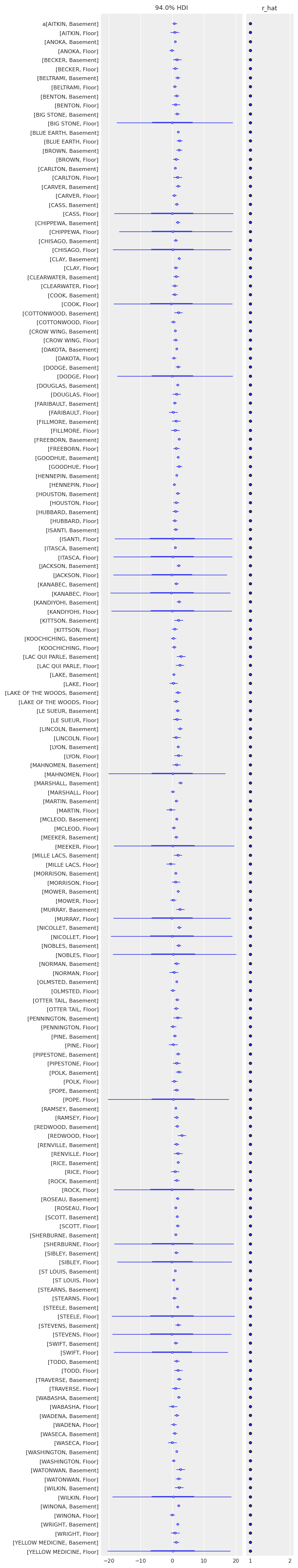
Sampling was good for all counties, but you can see that some are more uncertain than others, and all of these uncertain estimates are for floor measurements. This probably comes from the fact that some counties just have a handful of floor measurements, so the model is pretty uncertain about them.
To identify counties with high radon levels, we can plot the ordered mean estimates, as well as their 94% HPD:
unpooled_means = unpooled_idata.posterior.mean(dim=("chain", "draw"))
unpooled_hdi = az.hdi(unpooled_idata)
We will now take advantage of label based indexing for Datasets with the sel method and of automagical sorting capabilities. We first sort using the values of a specific 1D variable a. Then, thanks to unpooled_means and unpooled_hdi both having the County dimension, we can pass a 1D DataArray to sort the second dataset too.
fig, axes = plt.subplots(1, 2, figsize=(12, 5.5))
xticks = np.arange(0, 86, 6)
fontdict = {"horizontalalignment": "right", "fontsize": 10}
for ax, level in zip(axes, ["Basement", "Floor"]):
    unpooled_means_iter = unpooled_means.sel(Level=level).sortby("a")
    unpooled_hdi_iter = unpooled_hdi.sel(Level=level).sortby(unpooled_means_iter.a)
    unpooled_means_iter.plot.scatter(x="County", y="a", ax=ax, alpha=0.8)
    ax.vlines(
        np.arange(counties),
        unpooled_hdi_iter.a.sel(hdi="lower"),
        unpooled_hdi_iter.a.sel(hdi="higher"),
        color="orange",
        alpha=0.6,
    )
    ax.set(title=f"{level.title()} estimates", ylabel="Radon estimate", ylim=(-2, 4.5))
    ax.set_xticks(xticks)
    ax.set_xticklabels(unpooled_means_iter.County.values[xticks], fontdict=fontdict)
    ax.tick_params(rotation=30)
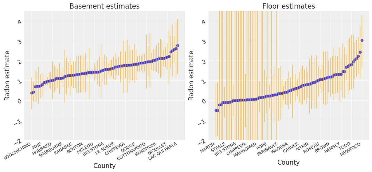
There seems to be more dispersion in radon levels for floor measurements than for basement ones. Moreover, as we saw in the forest plot, floor estimates are globally more uncertain, especially in some counties. We speculated that this is due to smaller sample sizes in the data, but let’s verify it!
n_floor_meas = srrs_mn.groupby("county").sum().floor
uncertainty = unpooled_hdi.a.sel(hdi="higher", Level="Floor") - unpooled_hdi.a.sel(
    hdi="lower", Level="Floor"
)

plt.plot(n_floor_meas, uncertainty, "o", alpha=0.4)
plt.xlabel("Nbr floor measurements in county")
plt.ylabel("Estimates' uncertainty");
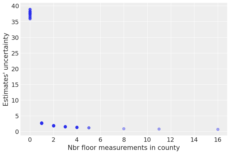
Bingo! This makes sense: it’s very hard to estimate floor radon levels in counties where there are no floor measurements, and the model is telling us that by being very uncertain in its estimates for those counties. This is a classic issue with no-pooling models: when you estimate clusters independently from each other, what do you with small-sample-size counties?
Another way to see this phenomenon is to visually compare the pooled and unpooled estimates for a subset of counties representing a range of sample sizes:
In cases where label based indexing is not powerful enough (for example when repeated labels are present) we can still index xarray objects with boolean masks or positional indices. Here we create a mask with the isin method and index with where. Note that xarray objects are generally high dimensional and condition based indexing is bound to generate ragged arrays. Thus, xarray.where by default replaces the unselected values with NaNs. In our case, the variable we are indexing is 1D and we can therefore use drop=True to remove the values instead of replacing by NaN.
Like we did above, we add a couple of extra coordinates to help in data processing and plotting.
SAMPLE_COUNTIES = (
    "LAC QUI PARLE",
    "AITKIN",
    "KOOCHICHING",
    "DOUGLAS",
    "CLAY",
    "STEARNS",
    "RAMSEY",
    "ST LOUIS",
)

unpooled_idata.observed_data = unpooled_idata.observed_data.assign_coords(
    {
        "County": ("obs_id", mn_counties[unpooled_idata.constant_data.county_idx]),
        "Level": (
            "obs_id",
            np.array(["Basement", "Floor"])[unpooled_idata.constant_data.floor_idx],
        ),
    }
)

fig, axes = plt.subplots(2, 4, figsize=(12, 6), sharey=True, sharex=True)
for ax, c in zip(axes.ravel(), SAMPLE_COUNTIES):
    sample_county_mask = unpooled_idata.observed_data.County.isin([c])

    # plot obs:
    unpooled_idata.observed_data.where(sample_county_mask, drop=True).sortby("Level").plot.scatter(
        x="Level", y="y", ax=ax, alpha=0.4
    )

    # plot both models:
    ax.plot([0, 1], unpooled_means.a.sel(County=c), "b")
    ax.plot([0, 1], pooled_means.a, "r--")

    ax.set_title(c)
    ax.set_xlabel("")
    ax.set_ylabel("Log radon level")
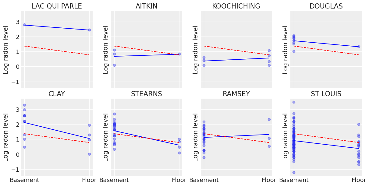
Neither of these models are satisfactory:
If we are trying to identify high-radon counties, pooling is useless – because, by definition, the pooled model estimates radon at the state-level. In other words, pooling leads to maximal underfitting: the variation across counties is not taken into account and only the overall population is estimated.
We do not trust extreme unpooled estimates produced by models using few observations. This leads to maximal overfitting: only the within-county variations are taken into account and the overall population (i.e the state-level, which tells us about similarites across counties) is not estimated.
This issue is acute for small sample sizes, as seen above: in counties where we have few floor measurements, if radon levels are higher for those data points than for basement ones (Aitkin, Koochiching, Ramsey), the model will estimate that radon levels are higher in floors than basements for these counties. But we shouldn’t trust this conclusion, because both scientific knowledge and the situation in other counties tell us that it is usually the reverse (basement radon > floor radon). So unless we have a lot of observations telling us otherwise for a given county, we should be skeptical and shrink our county-estimates to the state-estimates – in other words, we should balance between cluster-level and population-level information, and the amount of shrinkage will depend on how extreme and how numerous the data in each cluster are.
But how do we do that? Well, ladies and gentlemen, let me introduce you to… hierarchical models!
Multilevel and hierarchical models
When we pool our data, we imply that they are sampled from the same model. This ignores any variation among sampling units (other than sampling variance) – we assume that counties are all the same:

When we analyze data unpooled, we imply that they are sampled independently from separate models. At the opposite extreme from the pooled case, this approach claims that differences between sampling units are too large to combine them – we assume that counties have no similarity whatsoever:

In a hierarchical model, parameters are viewed as a sample from a population distribution of parameters. Thus, we view them as being neither entirely different or exactly the same. This is partial pooling:

We can use PyMC to easily specify multilevel models, and fit them using Markov chain Monte Carlo.
Partial pooling model
The simplest partial pooling model for the household radon dataset is one which simply estimates radon levels, without any predictors at any level. A partial pooling model represents a compromise between the pooled and unpooled extremes, approximately a weighted average (based on sample size) of the unpooled county estimates and the pooled estimates.
Estimates for counties with smaller sample sizes will shrink towards the state-wide average.
Estimates for counties with larger sample sizes will be closer to the unpooled county estimates and will influence the the state-wide average.
with pm.Model(coords=coords) as partial_pooling:
    county_idx = pm.Data("county_idx", county, dims="obs_id")
    # Hyperpriors:
    a = pm.Normal("a", mu=0.0, sigma=10.0)
    sigma_a = pm.Exponential("sigma_a", 1.0)

    # Varying intercepts:
    a_county = pm.Normal("a_county", mu=a, sigma=sigma_a, dims="County")

    # Expected value per county:
    theta = a_county[county_idx]
    # Model error:
    sigma = pm.Exponential("sigma", 1.0)

    y = pm.Normal("y", theta, sigma=sigma, observed=log_radon, dims="obs_id")
pm.model_to_graphviz(partial_pooling)

with partial_pooling:
    partial_pooling_idata = pm.sample(tune=2000, return_inferencedata=True, random_seed=RANDOM_SEED)
Auto-assigning NUTS sampler...
Initializing NUTS using jitter+adapt_diag...
Multiprocess sampling (4 chains in 4 jobs)
NUTS: [sigma, a_county, sigma_a, a]
Sampling 4 chains for 2_000 tune and 1_000 draw iterations (8_000 + 4_000 draws total) took 19 seconds.
The number of effective samples is smaller than 25% for some parameters.
To compare partial-pooling and no-pooling estimates, let’s run the unpooled model without the floor predictor:
with pm.Model(coords=coords) as unpooled_bis:
    county_idx = pm.Data("county_idx", county, dims="obs_id")
    a_county = pm.Normal("a_county", 0.0, sigma=10.0, dims="County")

    theta = a_county[county_idx]
    sigma = pm.Exponential("sigma", 1.0)

    y = pm.Normal("y", theta, sigma=sigma, observed=log_radon, dims="obs_id")

    unpooled_idata_bis = pm.sample(tune=2000, return_inferencedata=True, random_seed=RANDOM_SEED)
Auto-assigning NUTS sampler...
Initializing NUTS using jitter+adapt_diag...
Multiprocess sampling (4 chains in 4 jobs)
NUTS: [sigma, a_county]
Sampling 4 chains for 2_000 tune and 1_000 draw iterations (8_000 + 4_000 draws total) took 20 seconds.
Now let’s compare both models’ estimates for all 85 counties. We’ll plot the estimates against each county’s sample size, to let you see more clearly what hierarchical models bring to the table:
N_county = srrs_mn.groupby("county")["idnum"].count().values

fig, axes = plt.subplots(1, 2, figsize=(10, 4), sharex=True, sharey=True)
for ax, idata, level in zip(
    axes,
    (unpooled_idata_bis, partial_pooling_idata),
    ("no pooling", "partial pooling"),
):

    # add variable with x values to xarray dataset
    idata.posterior = idata.posterior.assign_coords({"N_county": ("County", N_county)})
    # plot means
    idata.posterior.mean(dim=("chain", "draw")).plot.scatter(
        x="N_county", y="a_county", ax=ax, alpha=0.9
    )
    ax.hlines(
        partial_pooling_idata.posterior.a.mean(),
        0.9,
        max(N_county) + 1,
        alpha=0.4,
        ls="--",
        label="Est. population mean",
    )

    # plot hdi
    hdi = az.hdi(idata).a_county
    ax.vlines(N_county, hdi.sel(hdi="lower"), hdi.sel(hdi="higher"), color="orange", alpha=0.5)

    ax.set(
        title=f"{level.title()} Estimates",
        xlabel="Nbr obs in county (log scale)",
        xscale="log",
        ylabel="Log radon",
    )
    ax.legend(fontsize=10)
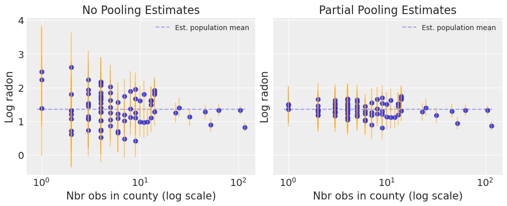
Notice the difference between the unpooled and partially-pooled estimates, particularly at smaller sample sizes: As expected, the former are both more extreme and more imprecise. Indeed, in the partially-pooled model, estimates in small-sample-size counties are informed by the population parameters – hence more precise estimates. Moreover, the smaller the sample size, the more regression towards the overall mean (the dashed gray line) – hence less extreme estimates. In other words, the model is skeptical of extreme deviations from the population mean in counties where data is sparse.
Now let’s try to integrate the floor predictor! To show you an example with a slope we’re gonna take the indicator variable road, but we could stay with the index variable approach that we used for the no-pooling model. Then we would have one intercept for each category – basement and floor.
Varying intercept model
As above, this model allows intercepts to vary across county, according to a random effect. We just add a fixed slope for the predictor (i.e all counties will have the same slope):
where
and the intercept random effect:
As with the the no-pooling model, we set a separate intercept for each county, but rather than fitting separate regression models for each county, multilevel modeling shares strength among counties, allowing for more reasonable inference in counties with little data. Here is what that looks in code:
with pm.Model(coords=coords) as varying_intercept:
    floor_idx = pm.Data("floor_idx", floor, dims="obs_id")
    county_idx = pm.Data("county_idx", county, dims="obs_id")
    # Hyperpriors:
    a = pm.Normal("a", mu=0.0, sigma=10.0)
    sigma_a = pm.Exponential("sigma_a", 1.0)

    # Varying intercepts:
    a_county = pm.Normal("a_county", mu=a, sigma=sigma_a, dims="County")
    # Common slope:
    b = pm.Normal("b", mu=0.0, sigma=10.0)

    # Expected value per county:
    theta = a_county[county_idx] + b * floor_idx
    # Model error:
    sigma = pm.Exponential("sigma", 1.0)

    y = pm.Normal("y", theta, sigma=sigma, observed=log_radon, dims="obs_id")
pm.model_to_graphviz(varying_intercept)

Let’s fit this bad boy with MCMC:
with varying_intercept:
    varying_intercept_idata = pm.sample(
        tune=2000, init="adapt_diag", random_seed=RANDOM_SEED, return_inferencedata=True
    )
Auto-assigning NUTS sampler...
Initializing NUTS using adapt_diag...
Multiprocess sampling (4 chains in 4 jobs)
NUTS: [sigma, b, a_county, sigma_a, a]
Sampling 4 chains for 2_000 tune and 1_000 draw iterations (8_000 + 4_000 draws total) took 27 seconds.
The number of effective samples is smaller than 25% for some parameters.
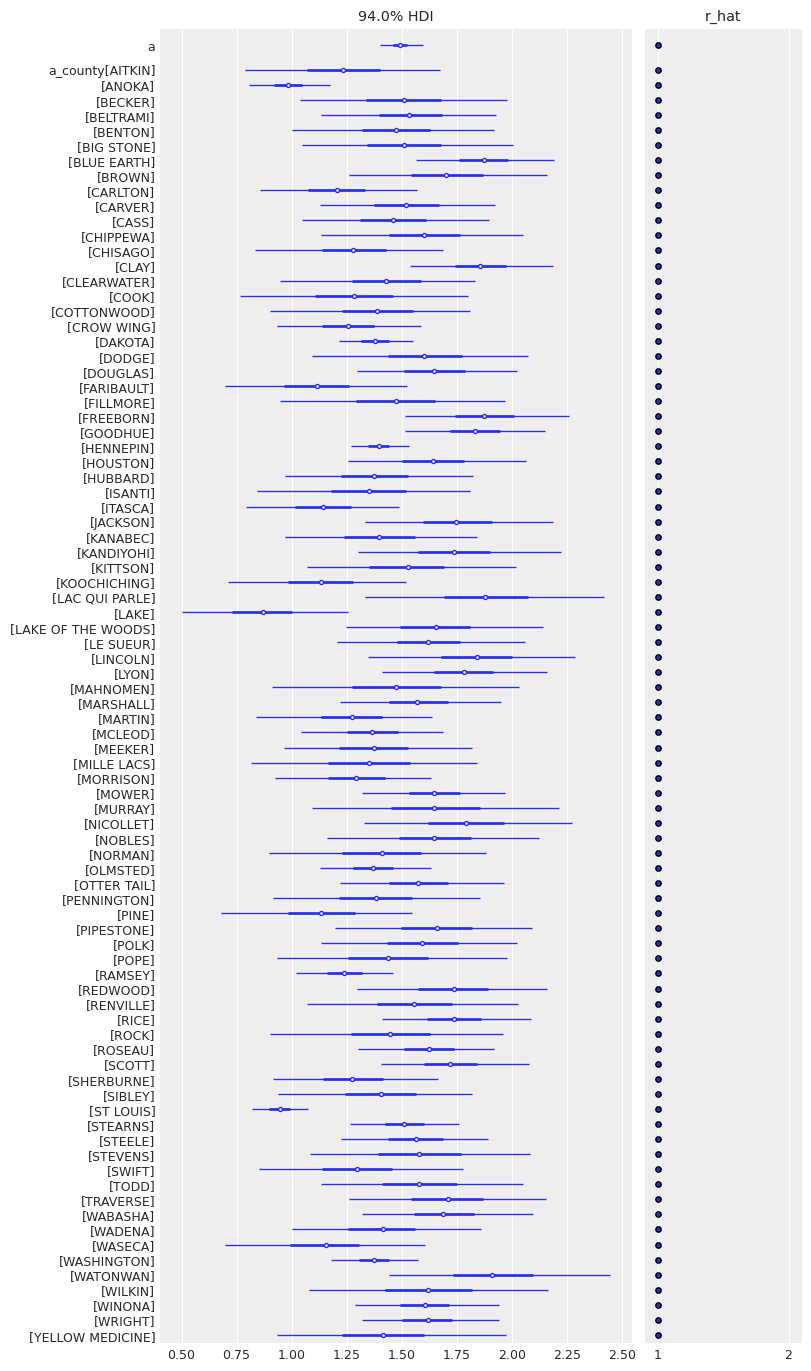
az.plot_forest(
    varying_intercept_idata, var_names=["a", "a_county"], r_hat=True, combined=True, textsize=9
);
az.plot_trace(varying_intercept_idata, var_names=["a", "sigma_a", "b", "sigma"]);
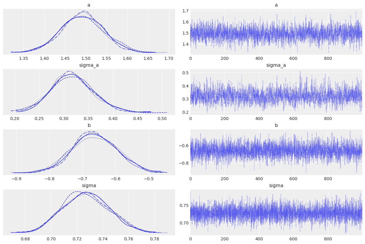
az.summary(varying_intercept_idata, var_names=["a", "sigma_a", "b", "sigma"], round_to=2)
| mean | sd | hdi_3% | hdi_97% | mcse_mean | mcse_sd | ess_bulk | ess_tail | r_hat | |
|---|---|---|---|---|---|---|---|---|---|
| a | 1.49 | 0.05 | 1.40 | 1.59 | 0.0 | 0.0 | 2001.69 | 2453.83 | 1.0 |
| sigma_a | 0.32 | 0.04 | 0.23 | 0.40 | 0.0 | 0.0 | 951.90 | 1092.09 | 1.0 |
| b | -0.66 | 0.07 | -0.78 | -0.53 | 0.0 | 0.0 | 3230.77 | 2984.59 | 1.0 |
| sigma | 0.73 | 0.02 | 0.69 | 0.76 | 0.0 | 0.0 | 5366.56 | 3088.67 | 1.0 |
As we suspected, the estimate for the floor coefficient is reliably negative and centered around -0.66. This can be interpreted as houses without basements having about half (\(\exp(-0.66) = 0.52\)) the radon levels of those with basements, after accounting for county. Note that this is only the relative effect of floor on radon levels: conditional on being in a given county, radon is expected to be half lower in houses without basements than in houses with. To see how much difference a basement makes on the absolute level of radon, we’d have to push the parameters through the model, as we do with posterior predictive checks and as we’ll do just now.
To do so, we will take advantage of automatic broadcasting with xarray. We want to create a 2D array with dimensions (County, Level), our variable a_county already has the County dimension. b however is a scalar. We will multiply b with an xvals DataArray to introduce the Level dimension into the mix. xarray will handle everything from there, no loops nor reshapings required.
xvals = xr.DataArray([0, 1], dims="Level", coords={"Level": ["Basement", "Floor"]})
post = varying_intercept_idata.posterior  # alias for readability
theta = (
    (post.a_county + post.b * xvals).mean(dim=("chain", "draw")).to_dataset(name="Mean log radon")
)

_, ax = plt.subplots()
theta.plot.scatter(x="Level", y="Mean log radon", alpha=0.2, color="k", ax=ax)  # scatter
ax.plot(xvals, theta["Mean log radon"].T, "k-", alpha=0.2)
# add lines too
ax.set_title("MEAN LOG RADON BY COUNTY");
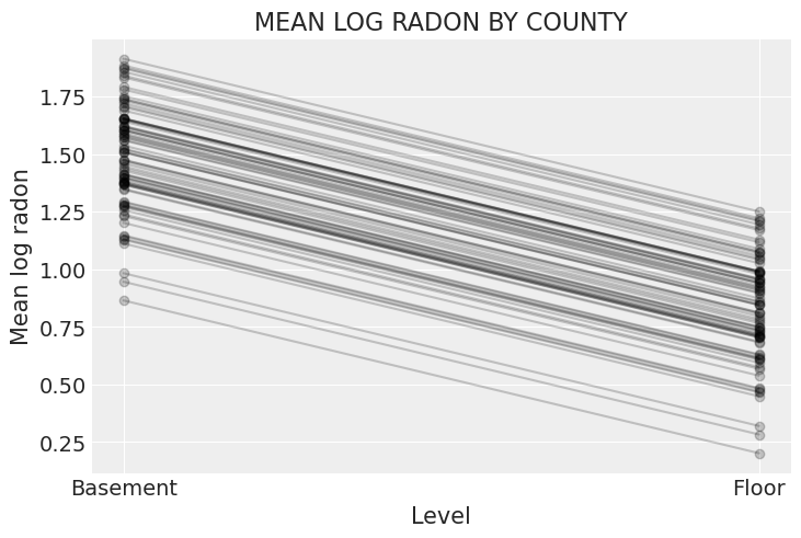
The graph above shows, for each county, the expected log radon level and the average effect of having no basement – these are the absolute effects we were talking about. Two caveats though:
This graph doesn’t show the uncertainty for each county – how confident are we that the average estimates are where the graph shows? For that we’d need to combine the uncertainty in
a_countyandb, and this would of course vary by county. I didn’t show it here because the graph would get cluttered, but go ahead and do it for a subset of counties.These are only average estimates at the county-level (
thetain the model): they don’t take into account the variation by household. To add this other layer of uncertainty we’d need to take stock of the effect ofsigmaand generate samples from theyvariable to see the effect on given households (that’s exactly the role of posterior predictive checks).
That being said, it is easy to show that the partial pooling model provides more objectively reasonable estimates than either the pooled or unpooled models, at least for counties with small sample sizes:
fig, axes = plt.subplots(2, 4, figsize=(12, 6), sharey=True, sharex=True)
for ax, c in zip(axes.ravel(), SAMPLE_COUNTIES):
    sample_county_mask = unpooled_idata.observed_data.County.isin([c])

    # plot obs:
    unpooled_idata.observed_data.where(sample_county_mask, drop=True).sortby("Level").plot.scatter(
        x="Level", y="y", ax=ax, alpha=0.4
    )

    # plot models:
    ax.plot([0, 1], unpooled_means.a.sel(County=c), "k:", alpha=0.5, label="No pooling")
    ax.plot([0, 1], pooled_means.a, "r--", label="Complete pooling")

    ax.plot([0, 1], theta["Mean log radon"].sel(County=c), "b", label="Partial pooling")

    ax.set_title(c)
    ax.set_xlabel("")
    ax.set_ylabel("")
    ax.tick_params(labelsize=10)

axes[0, 0].set_ylabel("Log radon level")
axes[1, 0].set_ylabel("Log radon level")
axes[0, 0].legend(fontsize=8, frameon=True), axes[1, 0].legend(fontsize=8, frameon=True);
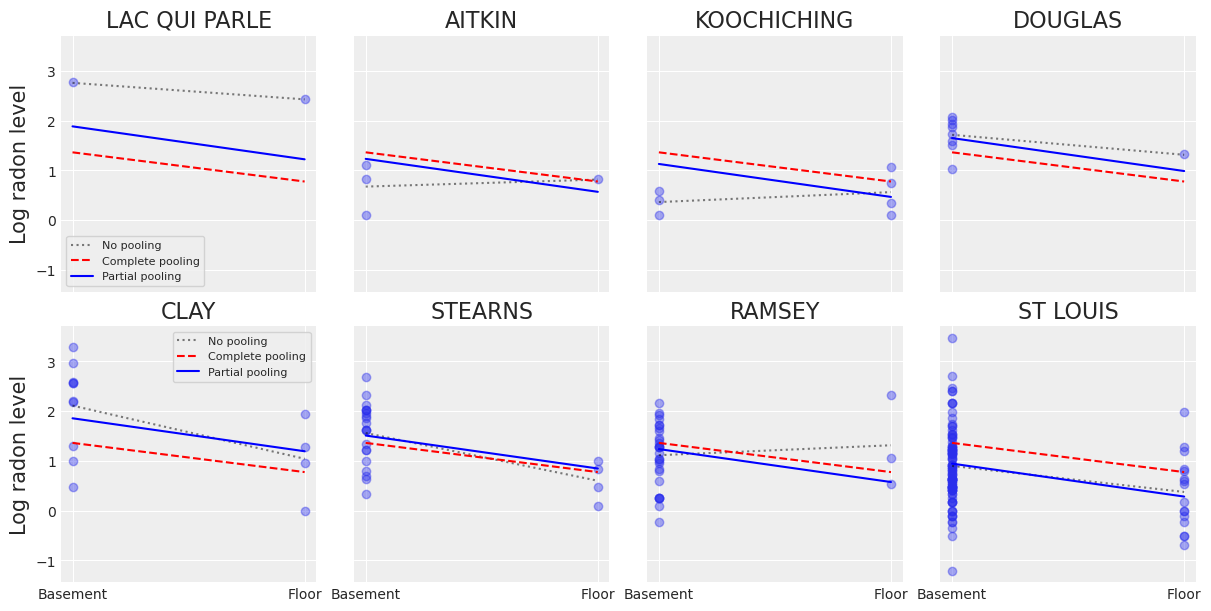
Here we clearly see the notion that partial-pooling is a compromise between no pooling and complete pooling, as its mean estimates are usually between the other models’ estimates. And interestingly, the bigger (smaller) the sample size in a given county, the closer the partial-pooling estimates are to the no-pooling (complete-pooling) estimates.
We see however that counties vary by more than just their baseline rates: the effect of floor seems to be different from one county to another. It would be great if our model could take that into account, wouldn’t it? Well to do that, we need to allow the slope to vary by county – not only the intercept – and here is how you can do it with PyMC3.
Varying intercept and slope model
The most general model allows both the intercept and slope to vary by county:
with pm.Model(coords=coords) as varying_intercept_slope:
    floor_idx = pm.Data("floor_idx", floor, dims="obs_id")
    county_idx = pm.Data("county_idx", county, dims="obs_id")

    # Hyperpriors:
    a = pm.Normal("a", mu=0.0, sigma=5.0)
    sigma_a = pm.Exponential("sigma_a", 1.0)
    b = pm.Normal("b", mu=0.0, sigma=1.0)
    sigma_b = pm.Exponential("sigma_b", 0.5)

    # Varying intercepts:
    a_county = pm.Normal("a_county", mu=a, sigma=sigma_a, dims="County")
    # Varying slopes:
    b_county = pm.Normal("b_county", mu=b, sigma=sigma_b, dims="County")

    # Expected value per county:
    theta = a_county[county_idx] + b_county[county_idx] * floor_idx
    # Model error:
    sigma = pm.Exponential("sigma", 1.0)

    y = pm.Normal("y", theta, sigma=sigma, observed=log_radon, dims="obs_id")
pm.model_to_graphviz(varying_intercept_slope)

Now, if you run this model, you’ll get divergences (some or a lot, depending on your random seed). We don’t want that – divergences are your Voldemort to your models. In these situations it’s usually wise to reparametrize your model using the “non-centered parametrization” (I know, it’s really not a great term, but please indulge me). We’re not gonna explain it here, but there are great resources out there. In a nutshell, it’s an algebraic trick that helps computation but leaves the model unchanged – the model is statistically equivalent to the “centered” version. In that case, here is what it would look like:
with pm.Model(coords=coords) as varying_intercept_slope:
    floor_idx = pm.Data("floor_idx", floor, dims="obs_id")
    county_idx = pm.Data("county_idx", county, dims="obs_id")

    # Hyperpriors:
    a = pm.Normal("a", mu=0.0, sigma=5.0)
    sigma_a = pm.Exponential("sigma_a", 1.0)
    b = pm.Normal("b", mu=0.0, sigma=1.0)
    sigma_b = pm.Exponential("sigma_b", 0.5)

    # Varying intercepts:
    za_county = pm.Normal("za_county", mu=0.0, sigma=1.0, dims="County")
    # Varying slopes:
    zb_county = pm.Normal("zb_county", mu=0.0, sigma=1.0, dims="County")

    # Expected value per county:
    theta = (a + za_county[county_idx] * sigma_a) + (b + zb_county[county_idx] * sigma_b) * floor
    # Model error:
    sigma = pm.Exponential("sigma", 1.0)

    y = pm.Normal("y", theta, sigma=sigma, observed=log_radon, dims="obs_id")

    varying_intercept_slope_idata = pm.sample(
        2000, tune=2000, target_accept=0.99, random_seed=RANDOM_SEED, return_inferencedata=True
    )
Auto-assigning NUTS sampler...
Initializing NUTS using jitter+adapt_diag...
Multiprocess sampling (4 chains in 4 jobs)
NUTS: [sigma, zb_county, za_county, sigma_b, b, sigma_a, a]
Sampling 4 chains for 2_000 tune and 2_000 draw iterations (8_000 + 8_000 draws total) took 118 seconds.
The number of effective samples is smaller than 25% for some parameters.
True, the code is uglier (for you, not for the computer), but:
The interpretation stays pretty much the same:
aandbare still the mean state-wide intercept and slope.sigma_aandsigma_bstill estimate the dispersion across counties of the intercepts and slopes (the more alike the counties, the smaller the corresponding sigma). The big change is that now the counties estimates (za_countyandzb_county) are z-scores. But the strategy to see what this means for mean radon levels per county is the same: push all these parameters through the model to get samples fromtheta.We don’t have any divergence: the model sampled more efficiently and converged more quickly than in the centered form.
Notice however that we had to increase the number of tuning steps. Looking at the trace helps us understand why:
az.plot_trace(varying_intercept_slope_idata, compact=True, chain_prop={"ls": "-"});
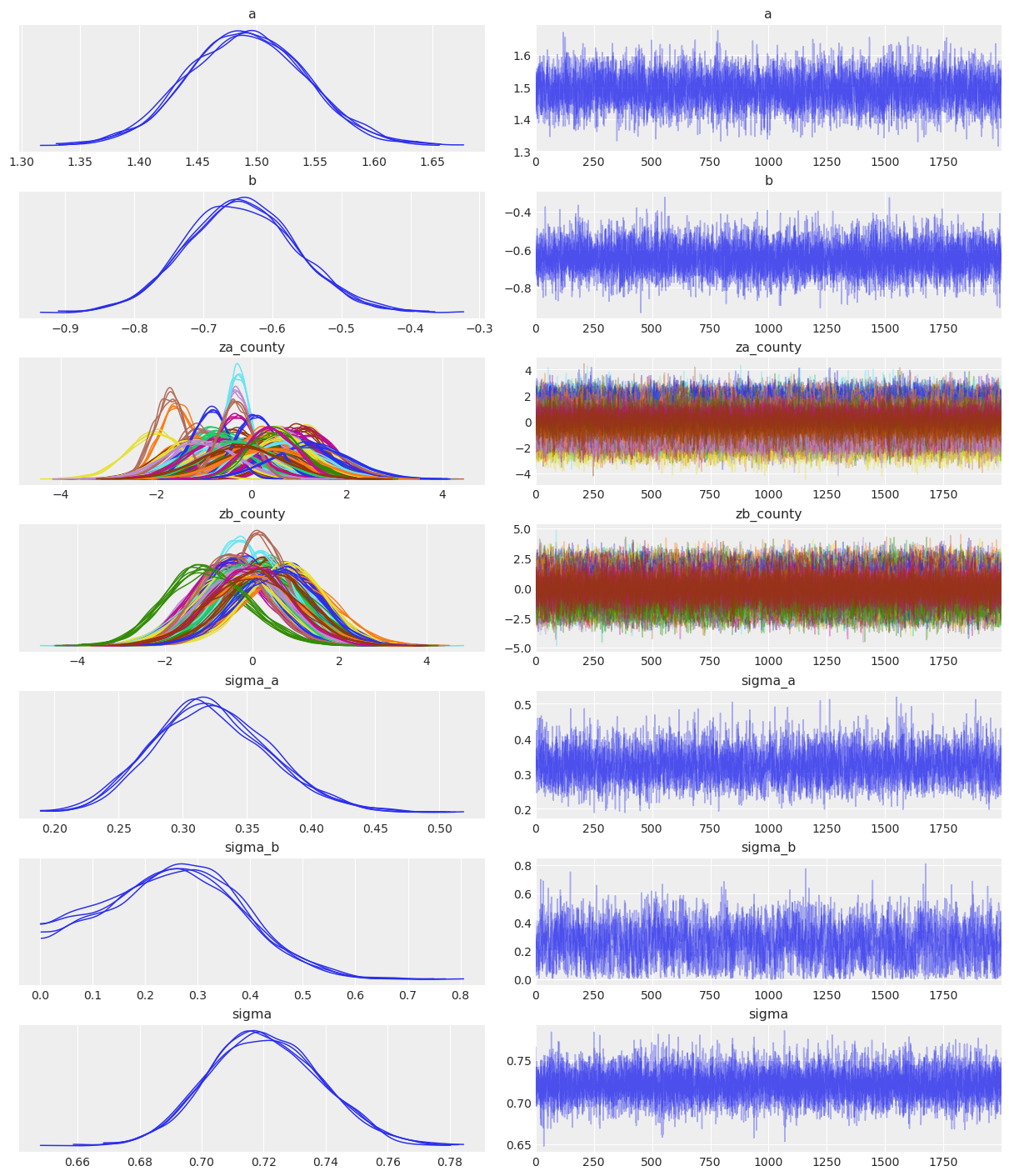
All chains look good and we get a negative b coefficient, illustrating the mean downward effect of no-basement on radon levels at the state level. But notice that sigma_b often gets very near zero – which would indicate that counties don’t vary that much in their answer to the floor “treatment”. That’s probably what bugged MCMC when using the centered parametrization: these situations usually yield a weird geometry for the sampler, causing the divergences. In other words, the non-centered form often perfoms better when one of the sigmas gets close to zero. But here, even with the non-centered model the sampler is not that comfortable with sigma_b: in fact if you look at the estimates with az.summary you’ll probably see that the number of effective samples is quite low for sigma_b.
Also note that sigma_a is not that big either – i.e counties do differ in their baseline radon levels, but not by a lot. However we don’t have that much of a problem to sample from this distribution because it’s much narrower than sigma_b and doesn’t get dangerously close to 0.
To wrap up this model, let’s plot the relationship between radon and floor for each county:
xvals = xr.DataArray([0, 1], dims="Level", coords={"Level": ["Basement", "Floor"]})
post = varying_intercept_slope_idata.posterior  # alias for readability
avg_a_county = (post.a + post.za_county * post.sigma_a).mean(dim=("chain", "draw"))
avg_b_county = (post.b + post.zb_county * post.sigma_b).mean(dim=("chain", "draw"))
theta = (avg_a_county + avg_b_county * xvals).to_dataset(name="Mean log radon")

_, ax = plt.subplots()
theta.plot.scatter(x="Level", y="Mean log radon", alpha=0.2, color="k", ax=ax)  # scatter
ax.plot(xvals, theta["Mean log radon"].T, "k-", alpha=0.2)
# add lines too
ax.set_title("MEAN LOG RADON BY COUNTY");
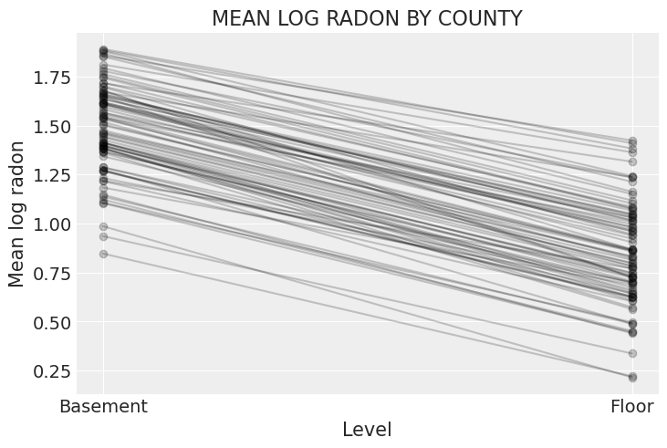
With the same caveats as earlier, we can see that now both the intercept and the slope vary by county – and isn’t that a marvel of statistics? But wait, there is more! We can (and maybe should) take into account the covariation between intercepts and slopes: when baseline radon is low in a given county, maybe that means the difference between floor and basement measurements will decrease – because there isn’t that much radon anyway. That would translate into a positive correlation between a_county and b_county, and adding that into our model would make even more efficient use the available data.
Or maybe the correlation is negative? In any case, we can’t know that unless we model it. To do that, we’ll use a multivariate Normal distribution instead of two different Normals for a_county and b_county. This simply means that each county’s parameters come from a common distribution with mean a for intercepts and b for slopes, and slopes and intercepts co-vary according to the covariance matrix S. In mathematical form:
where \(\alpha\) and \(\beta\) are the mean intercept and slope respectively, \(\sigma_{\alpha}\) and \(\sigma_{\beta}\) represent the variation in intercepts and slopes respectively, and \(P\) is the correlation matrix of intercepts and slopes. In this case, as their is only one slope, \(P\) contains only one relevant figure: the correlation between \(\alpha\) and \(\beta\).
This translates quite easily in PyMC3:
coords["param"] = ["a", "b"]
coords["param_bis"] = ["a", "b"]
with pm.Model(coords=coords) as covariation_intercept_slope:
    floor_idx = pm.Data("floor_idx", floor, dims="obs_id")
    county_idx = pm.Data("county_idx", county, dims="obs_id")

    # prior stddev in intercepts & slopes (variation across counties):
    sd_dist = pm.Exponential.dist(0.5)

    # get back standard deviations and rho:
    chol, corr, stds = pm.LKJCholeskyCov("chol", n=2, eta=2.0, sd_dist=sd_dist, compute_corr=True)

    # prior for average intercept:
    a = pm.Normal("a", mu=0.0, sigma=5.0)
    # prior for average slope:
    b = pm.Normal("b", mu=0.0, sigma=1.0)
    # population of varying effects:
    ab_county = pm.MvNormal("ab_county", mu=tt.stack([a, b]), chol=chol, dims=("County", "param"))

    # Expected value per county:
    theta = ab_county[county_idx, 0] + ab_county[county_idx, 1] * floor_idx
    # Model error:
    sigma = pm.Exponential("sigma", 1.0)

    y = pm.Normal("y", theta, sigma=sigma, observed=log_radon, dims="obs_id")
pm.model_to_graphviz(covariation_intercept_slope)

This is by far the most complex model we’ve done so far, so it’s normal if you’re confused. Just take some time to let it sink in. The centered version mirrors the mathematical notions very closely, so you should be able to get the gist of it. Of course, you guessed it, we’re gonna need the non-centered version. There is actually just one change:
with pm.Model(coords=coords) as covariation_intercept_slope:
    floor_idx = pm.Data("floor_idx", floor, dims="obs_id")
    county_idx = pm.Data("county_idx", county, dims="obs_id")

    # prior stddev in intercepts & slopes (variation across counties):
    sd_dist = pm.Exponential.dist(0.5)

    # get back standard deviations and rho:
    chol, corr, stds = pm.LKJCholeskyCov("chol", n=2, eta=2.0, sd_dist=sd_dist, compute_corr=True)

    # prior for average intercept:
    a = pm.Normal("a", mu=0.0, sigma=5.0)
    # prior for average slope:
    b = pm.Normal("b", mu=0.0, sigma=1.0)
    # population of varying effects:
    z = pm.Normal("z", 0.0, 1.0, dims=("param", "County"))
    ab_county = pm.Deterministic("ab_county", tt.dot(chol, z).T, dims=("County", "param"))

    # Expected value per county:
    theta = a + ab_county[county_idx, 0] + (b + ab_county[county_idx, 1]) * floor_idx
    # Model error:
    sigma = pm.Exponential("sigma", 1.0)

    y = pm.Normal("y", theta, sigma=sigma, observed=log_radon, dims="obs_id")

    covariation_intercept_slope_idata = pm.sample(
        2000,
        tune=2000,
        target_accept=0.99,
        random_seed=RANDOM_SEED,
        return_inferencedata=True,
        idata_kwargs={"dims": {"chol_stds": ["param"], "chol_corr": ["param", "param_bis"]}},
    )
Auto-assigning NUTS sampler...
Initializing NUTS using jitter+adapt_diag...
Multiprocess sampling (4 chains in 4 jobs)
NUTS: [sigma, z, b, a, chol]
Sampling 4 chains for 2_000 tune and 2_000 draw iterations (8_000 + 8_000 draws total) took 290 seconds.
The number of effective samples is smaller than 25% for some parameters.
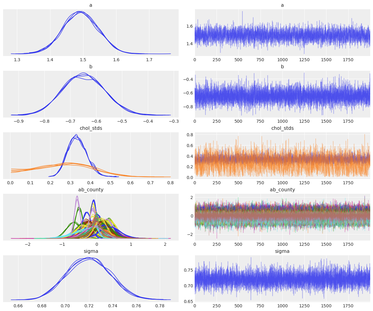
az.plot_trace(
    covariation_intercept_slope_idata,
    var_names=["~z", "~chol", "~chol_corr"],
    compact=True,
    chain_prop={"ls": "-"},
);
az.plot_trace(
    covariation_intercept_slope_idata,
    var_names="chol_corr",
    lines=[("chol_corr", {}, 0.0)],
    compact=True,
    chain_prop={"ls": "-"},
    coords={
        "param": xr.DataArray(["a"], dims=["pointwise_sel"]),
        "param_bis": xr.DataArray(["b"], dims=["pointwise_sel"]),
    },
);
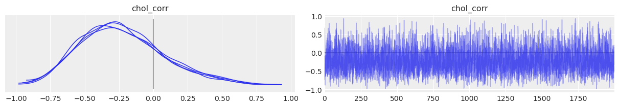
So the correlation between slopes and intercepts seems to be negative: when a_county increases, b_county tends to decrease. In other words, when basement radon in a county gets bigger, the difference with floor radon tends to get bigger too (because floor readings get smaller while basement readings get bigger). But again, the uncertainty is wide on Rho so it’s possible the correlation goes the other way around or is simply close to zero.
And how much variation is there across counties? It’s not easy to read sigma_ab above, so let’s do a forest plot and compare the estimates with the model that doesn’t include the covariation between slopes and intercepts:
az.plot_forest(
    [varying_intercept_slope_idata, covariation_intercept_slope_idata],
    model_names=["No covariation", "With covariation"],
    var_names=["a", "b", "sigma_a", "sigma_b", "chol_stds", "chol_corr"],
    combined=True,
    figsize=(8, 6),
);
The estimates are very close to each other, both for the means and the standard deviations. But remember, the information given by Rho is only seen at the county level: in theory it uses even more information from the data to get an even more informed pooling of information for all county parameters. So let’s visually compare estimates of both models at the county level:
# posterior means of covariation model:
a_county_cov = (
    covariation_intercept_slope_idata.posterior["a"]
    + covariation_intercept_slope_idata.posterior["ab_county"].sel(param="a")
).mean(dim=("chain", "draw"))
b_county_cov = (
    covariation_intercept_slope_idata.posterior["b"]
    + covariation_intercept_slope_idata.posterior["ab_county"].sel(param="b")
).mean(dim=("chain", "draw"))

# plot both and connect with lines
plt.scatter(avg_a_county, avg_b_county, label="No cov estimates", alpha=0.6)
plt.scatter(
    a_county_cov,
    b_county_cov,
    facecolors="none",
    edgecolors="k",
    lw=1,
    label="With cov estimates",
    alpha=0.8,
)
plt.plot([avg_a_county, a_county_cov], [avg_b_county, b_county_cov], "k-", alpha=0.5)
plt.xlabel("Intercept")
plt.ylabel("Slope")
plt.legend();
The negative correlation is somewhat clear here: when the intercept increases, the slope decreases. So we understand why the model put most of the posterior weight into negative territory for Rho. Nevertheless, the negativity isn’t that obvious, which is why the model gives a non-trivial posterior probability to the possibility that Rho could in fact be zero or positive.
Interestingly, the differences between both models occur at extreme slope and intercept values. This is because the second model used the slightly negative correlation between intercepts and slopes to adjust their estimates: when intercepts are larger (smaller) than average, the model pushes down (up) the associated slopes.
Globally, there is a lot of agreement here: modeling the correlation didn’t change inference that much. We already saw that radon levels tended to be lower in floors than basements, and when we checked the posterior distributions of the average effects (a and b) and standard deviations, we noticed that they were almost identical. But on average the model with covariation will be more accurate – because it squeezes additional information from the data, to shrink estimates in both dimensions.
Adding group-level predictors
A primary strength of multilevel models is the ability to handle predictors on multiple levels simultaneously. If we consider the varying-intercepts model above:
we may, instead of a simple random effect to describe variation in the expected radon value, specify another regression model with a county-level covariate. Here, we use the county uranium reading \(u_j\), which is thought to be related to radon levels:
Thus, we are now incorporating a house-level predictor (floor or basement) as well as a county-level predictor (uranium).
Note that the model has both indicator variables for each county, plus a county-level covariate. In classical regression, this would result in collinearity. In a multilevel model, the partial pooling of the intercepts towards the expected value of the group-level linear model avoids this.
Group-level predictors also serve to reduce group-level variation, \(\sigma_{\alpha}\) (here it would be the variation across counties, sigma_a). An important implication of this is that the group-level estimate induces stronger pooling – by definition, a smaller \(\sigma_{\alpha}\) means a stronger shrinkage of counties parameters towards the overall state mean.
This is fairly straightforward to implement in PyMC3 – we just add another level:
with pm.Model(coords=coords) as hierarchical_intercept:
    floor_idx = pm.Data("floor_idx", floor, dims="obs_id")
    county_idx = pm.Data("county_idx", county, dims="obs_id")
    uranium = pm.Data("uranium", u, dims="County")

    # Hyperpriors:
    g = pm.Normal("g", mu=0.0, sigma=10.0, shape=2)
    sigma_a = pm.Exponential("sigma_a", 1.0)

    # Varying intercepts uranium model:
    a = g[0] + g[1] * uranium
    a_county = pm.Normal("a_county", mu=a, sigma=sigma_a, dims="County")
    # Common slope:
    b = pm.Normal("b", mu=0.0, sigma=1.0)

    # Expected value per county:
    theta = a_county[county_idx] + b * floor_idx
    # Model error:
    sigma = pm.Exponential("sigma", 1.0)

    y = pm.Normal("y", theta, sigma=sigma, observed=log_radon, dims="obs_id")
pm.model_to_graphviz(hierarchical_intercept)

Do you see the new level, with sigma_a and g, which is two-dimensional because it contains the linear model for a_county? Now, if we run this model we’re gonna get… divergences, you guessed it! So we’re gonna switch to the non-centered form again:
with pm.Model(coords=coords) as hierarchical_intercept:
    floor_idx = pm.Data("floor_idx", floor, dims="obs_id")
    county_idx = pm.Data("county_idx", county, dims="obs_id")
    uranium = pm.Data("uranium", u, dims="County")

    # Hyperpriors:
    g = pm.Normal("g", mu=0.0, sigma=10.0, shape=2)
    sigma_a = pm.Exponential("sigma_a", 1.0)

    # Varying intercepts uranium model:
    a = pm.Deterministic("a", g[0] + g[1] * uranium, dims="County")
    za_county = pm.Normal("za_county", mu=0.0, sigma=1.0, dims="County")
    a_county = pm.Deterministic("a_county", a + za_county * sigma_a, dims="County")
    # Common slope:
    b = pm.Normal("b", mu=0.0, sigma=1.0)

    # Expected value per county:
    theta = a_county[county_idx] + b * floor_idx
    # Model error:
    sigma = pm.Exponential("sigma", 1.0)

    y = pm.Normal("y", theta, sigma=sigma, observed=log_radon, dims="obs_id")

    hierarchical_intercept_idata = pm.sample(
        2000, tune=2000, target_accept=0.99, random_seed=RANDOM_SEED, return_inferencedata=True
    )
Auto-assigning NUTS sampler...
Initializing NUTS using jitter+adapt_diag...
Multiprocess sampling (4 chains in 4 jobs)
NUTS: [sigma, b, za_county, sigma_a, g]
Sampling 4 chains for 2_000 tune and 2_000 draw iterations (8_000 + 8_000 draws total) took 66 seconds.
The number of effective samples is smaller than 25% for some parameters.
uranium = hierarchical_intercept_idata.constant_data.uranium
post = hierarchical_intercept_idata.posterior.assign_coords(uranium=uranium)
avg_a = post["a"].mean(dim=("chain", "draw")).sortby("uranium")
avg_a_county = post["a_county"].mean(dim=("chain", "draw"))
avg_a_county_hdi = az.hdi(post, var_names="a_county")["a_county"]

_, ax = plt.subplots()
ax.plot(avg_a.uranium, avg_a, "k--", alpha=0.6, label="Mean intercept")
az.plot_hdi(
    uranium,
    post["a"],
    fill_kwargs={"alpha": 0.1, "color": "k", "label": "Mean intercept HPD"},
    ax=ax,
)
ax.scatter(uranium, avg_a_county, alpha=0.8, label="Mean county-intercept")
ax.vlines(
    uranium,
    avg_a_county_hdi.sel(hdi="lower"),
    avg_a_county_hdi.sel(hdi="higher"),
    alpha=0.5,
    color="orange",
)
plt.xlabel("County-level uranium")
plt.ylabel("Intercept estimate")
plt.legend(fontsize=9);
Uranium is indeed much associated with baseline radon levels in each county. The graph above shows the average relationship and its uncertainty: the baseline radon level in an average county as a function of uranium, as well as the 94% HPD of this radon level (grey line and envelope). The blue points and orange bars represent the relationship between baseline radon and uranium, but now for each county. As you see, the uncertainty is bigger now, because it adds on top of the average uncertainty – each county has its idyosyncracies after all.
If we compare the county-intercepts for this model with those of the partial-pooling model without a county-level covariate:
az.plot_forest(
    [varying_intercept_idata, hierarchical_intercept_idata],
    model_names=["W/t. county pred.", "With county pred."],
    var_names=["a_county"],
    combined=True,
    figsize=(6, 40),
    textsize=9,
);
We see that the compatibility intervals are narrower for the model including the county-level covariate. This is expected, as the effect of a covariate is to reduce the variation in the outcome variable – provided the covariate is of predictive value. More importantly, with this model we were able to squeeze even more information out of the data.
Correlations among levels
In some instances, having predictors at multiple levels can reveal correlation between individual-level variables and group residuals. We can account for this by including the average of the individual predictors as a covariate in the model for the group intercept:
These are broadly referred to as contextual effects.
To add these effects to our model, let’s create a new variable containing the mean of floor in each county and add that to our previous model:
avg_floor_data = srrs_mn.groupby("county")["floor"].mean().rename(county_lookup).values

with pm.Model(coords=coords) as contextual_effect:
    floor_idx = pm.Data("floor_idx", floor, dims="obs_id")
    county_idx = pm.Data("county_idx", county, dims="obs_id")
    uranium = pm.Data("uranium", u, dims="County")
    avg_floor = pm.Data("avg_floor", avg_floor_data, dims="County")

    # Hyperpriors:
    g = pm.Normal("g", mu=0.0, sigma=10.0, shape=3)
    sigma_a = pm.Exponential("sigma_a", 1.0)

    # Varying intercepts uranium model:
    a = pm.Deterministic("a", g[0] + g[1] * u + g[2] * avg_floor, dims="County")
    za_county = pm.Normal("za_county", mu=0.0, sigma=1.0, dims="County")
    a_county = pm.Deterministic("a_county", a + za_county * sigma_a, dims="County")
    # Common slope:
    b = pm.Normal("b", mu=0.0, sigma=1.0)

    # Expected value per county:
    theta = a_county[county_idx] + b * floor_idx
    # Model error:
    sigma = pm.Exponential("sigma", 1.0)

    y = pm.Normal("y", theta, sigma=sigma, observed=log_radon, dims="obs_id")

    contextual_effect_idata = pm.sample(
        2000, tune=2000, target_accept=0.99, random_seed=RANDOM_SEED, return_inferencedata=True
    )
Auto-assigning NUTS sampler...
Initializing NUTS using jitter+adapt_diag...
Multiprocess sampling (4 chains in 4 jobs)
NUTS: [sigma, b, za_county, sigma_a, g]
Sampling 4 chains for 2_000 tune and 2_000 draw iterations (8_000 + 8_000 draws total) took 87 seconds.
The number of effective samples is smaller than 25% for some parameters.
az.summary(contextual_effect_idata, var_names=["g"], round_to=2)
| mean | sd | hdi_3% | hdi_97% | mcse_mean | mcse_sd | ess_bulk | ess_tail | r_hat | |
|---|---|---|---|---|---|---|---|---|---|
| g[0] | 1.43 | 0.05 | 1.34 | 1.52 | 0.0 | 0.0 | 3848.43 | 4886.02 | 1.0 |
| g[1] | 0.70 | 0.09 | 0.54 | 0.86 | 0.0 | 0.0 | 4996.25 | 5415.66 | 1.0 |
| g[2] | 0.39 | 0.20 | 0.02 | 0.76 | 0.0 | 0.0 | 4460.20 | 5349.41 | 1.0 |
So we might infer from this that counties with higher proportions of houses without basements tend to have higher baseline levels of radon. This seems to be new, as up to this point we saw that floor was negatively associated with radon levels. But remember this was at the household-level: radon tends to be higher in houses with basements. But at the county-level it seems that the less basements on average in the county, the more radon. So it’s not that contradictory. What’s more, the estimate for \(\gamma_2\) is quite uncertain and overlaps with zero, so it’s possible that the relationship is not that strong. And finally, let’s note that \(\gamma_2\) estimates something else than uranium’s effect, as this is already taken into account by \(\gamma_1\) – it answers the question “once we know uranium level in the county, is there any value in learning about the proportion of houses without basements?”.
All of this is to say that we shouldn’t interpret this causally: there is no credible mecanism by which a basement (or absence thereof) causes radon emissions. More probably, our causal graph is missing something: a confounding variable, one that influences both basement construction and radon levels, is lurking somewhere in the dark… Perhaps is it the type of soil, which might influence what type of structures are built and the level of radon? Maybe adding this to our model would help with causal inference.
Prediction
Gelman (2006) used cross-validation tests to check the prediction error of the unpooled, pooled, and partially-pooled models
root mean squared cross-validation prediction errors:
unpooled = 0.86
pooled = 0.84
multilevel = 0.79
There are two types of prediction that can be made in a multilevel model:
a new individual within an existing group
a new individual within a new group
The first type is the easiest one, as we’ve generally already sampled from the existing group. For this model, the first type of posterior prediction is the only one making sense, as counties are not added or deleted every day. So, if we wanted to make a prediction for, say, a new house with no basement in St. Louis and Kanabec counties, we just need to sample from the radon model with the appropriate intercept:
county_lookup["ST LOUIS"], county_lookup["KANABEC"]
(69, 31)
That is,
Because we judiciously set the county index and floor values as shared variables earlier, we can modify them directly to the desired values (69 and 1 respectively) and sample corresponding posterior predictions, without having to redefine and recompile our model. Using the model just above:
prediction_coords = {"obs_id": ["ST LOUIS", "KANABEC"]}
with contextual_effect:
    pm.set_data({"county_idx": np.array([69, 31]), "floor_idx": np.array([1, 1])})
    stl_pred = pm.fast_sample_posterior_predictive(
        contextual_effect_idata.posterior, random_seed=RANDOM_SEED
    )
    az.from_pymc3_predictions(
        stl_pred, idata_orig=contextual_effect_idata, inplace=True, coords=prediction_coords
    )
az.plot_posterior(contextual_effect_idata, group="predictions");
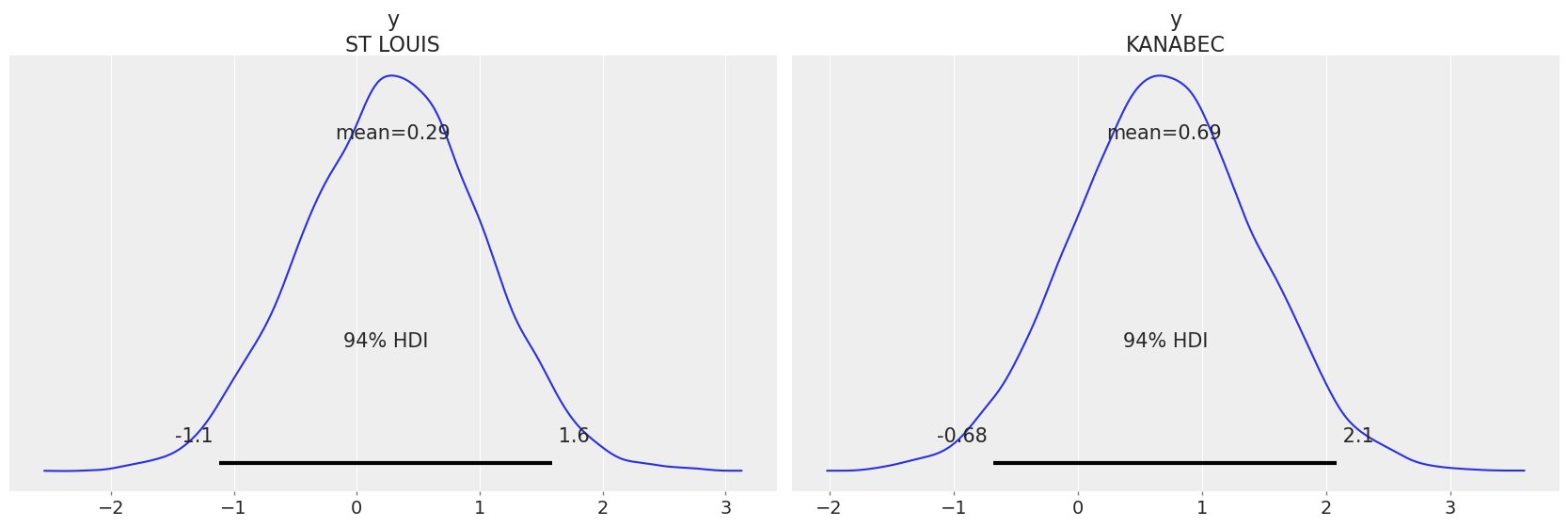
Benefits of Multilevel Models
Accounting for natural hierarchical structure of observational data.
Estimation of coefficients for (under-represented) groups.
Incorporating individual- and group-level information when estimating group-level coefficients.
Allowing for variation among individual-level coefficients across groups.
References
- 1
Andrew Gelman and Jennifer Hill. Data analysis using regression and multilevel/hierarchical models. Cambridge university press, 2006.
- 2
Richard McElreath. Statistical rethinking: A Bayesian course with examples in R and Stan. Chapman and Hall/CRC, 2018.
- 3
Andrew Gelman. Multilevel (hierarchical) modeling: what it can and cannot do. Technometrics, 48(3):432–435, 2006.
Watermark
%load_ext watermark
%watermark -n -u -v -iv -w
Last updated: Sun Nov 14 2021

Python implementation: CPython
Python version       : 3.9.7
IPython version      : 7.29.0

arviz     : 0.11.4
numpy     : 1.21.3
pymc3     : 3.11.4
xarray    : 0.20.0
sys       : 3.9.7 | packaged by conda-forge | (default, Sep 29 2021, 20:33:18)
[Clang 11.1.0 ]
theano    : 1.1.2
matplotlib: 3.4.3
pandas    : 1.3.4

Watermark: 2.2.0
- Chris Fonnesbeck , Colin Carroll , Alex Andorra , Oriol Abril , Farhan Reynaldo . "A Primer on Bayesian Methods for Multilevel Modeling". In: PyMC Examples. Ed. by PyMC Team. DOI: 10.5281/zenodo.5832070