Modeling Heteroscedasticity with BART

In this notebook we show how to use BART to model heteroscedasticity as described in Section 4.1 of pymc-bart’s paper []. We use the marketing data set provided by the R package datarium []. The idea is to model a marketing channel contribution to sales as a function of budget.

import os

import arviz as az
import matplotlib.pyplot as plt
import numpy as np
import pandas as pd
import pymc as pm
import pymc_bart as pmb

%config InlineBackend.figure_format = "retina"
az.style.use("arviz-darkgrid")
plt.rcParams["figure.figsize"] = [10, 6]
rng = np.random.default_rng(42)

Read Data

try:
    df = pd.read_csv(os.path.join("..", "data", "marketing.csv"), sep=";", decimal=",")
except FileNotFoundError:
    df = pd.read_csv(pm.get_data("marketing.csv"), sep=";", decimal=",")

n_obs = df.shape[0]

df.head()

	youtube	facebook	newspaper	sales
0	276.12	45.36	83.04	26.52
1	53.40	47.16	54.12	12.48
2	20.64	55.08	83.16	11.16
3	181.80	49.56	70.20	22.20
4	216.96	12.96	70.08	15.48

EDA

We start by looking into the data. We are going to focus on Youtube.

fig, ax = plt.subplots()
ax.plot(df["youtube"], df["sales"], "o", c="C0")
ax.set(title="Sales as a function of Youtube budget", xlabel="budget", ylabel="sales");

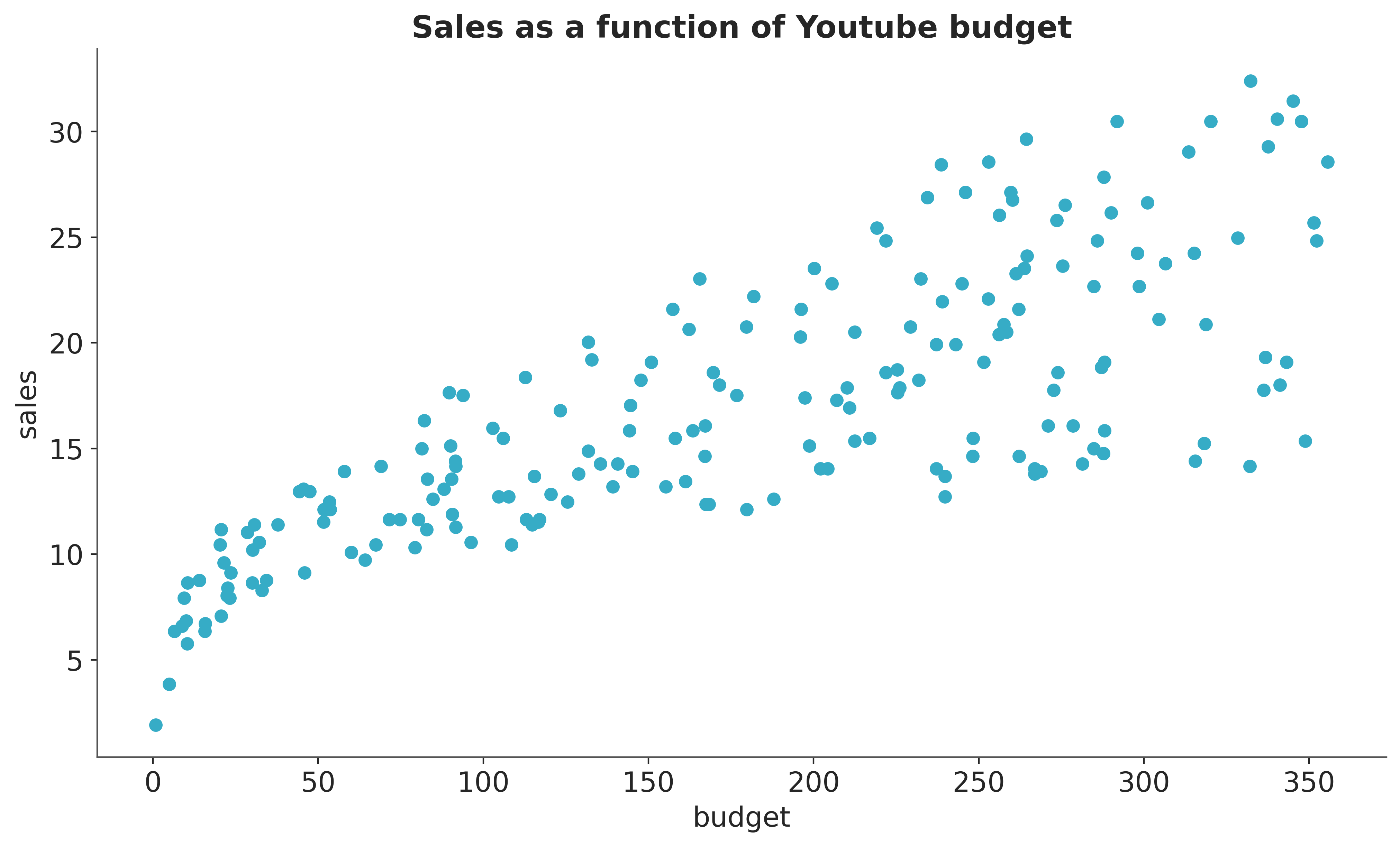
We clearly see that both the mean and variance are increasing as a function of budget. One possibility is to manually select an explicit parametrization of these functions, e.g. square root or logarithm. However, in this example we want to learn these functions from the data using a BART model.

Model Specification

We proceed to prepare the data for modeling. We are going to use the budget as the predictor and sales as the response.

X = df["youtube"].to_numpy().reshape(-1, 1)
Y = df["sales"].to_numpy()

Next, we specify the model. Note that we just need one BART distribution which can be vectorized to model both the mean and variance. We use a Gamma distribution as likelihood as we expect the sales to be positive.

with pm.Model() as model_marketing_full:
    w = pmb.BART("w", X=X, Y=np.log(Y), m=100, shape=(2, n_obs))
    y = pm.Gamma("y", mu=pm.math.exp(w[0]), sigma=pm.math.exp(w[1]), observed=Y)

pm.model_to_graphviz(model=model_marketing_full)

We now fit the model.

with model_marketing_full:
    idata_marketing_full = pm.sample(2000, random_seed=rng, compute_convergence_checks=False)
    posterior_predictive_marketing_full = pm.sample_posterior_predictive(
        trace=idata_marketing_full, random_seed=rng
    )

Multiprocess sampling (4 chains in 4 jobs)
PGBART: [w]

100.00% [12000/12000 02:25<00:00 Sampling 4 chains, 0 divergences]

Sampling 4 chains for 1_000 tune and 2_000 draw iterations (4_000 + 8_000 draws total) took 145 seconds.
Sampling: [y]

100.00% [8000/8000 00:00<00:00]

Results

We can now visualize the posterior predictive distribution of the mean and the likelihood.

posterior_mean = idata_marketing_full.posterior["w"].mean(dim=("chain", "draw"))[0]

w_hdi = az.hdi(ary=idata_marketing_full, group="posterior", var_names=["w"], hdi_prob=0.5)

pps = az.extract(
    posterior_predictive_marketing_full, group="posterior_predictive", var_names=["y"]
).T

idx = np.argsort(X[:, 0])


fig, ax = plt.subplots()
az.plot_hdi(
    x=X[:, 0],
    y=pps,
    ax=ax,
    hdi_prob=0.90,
    fill_kwargs={"alpha": 0.3, "label": r"Observations $90\%$ HDI"},
)
az.plot_hdi(
    x=X[:, 0],
    hdi_data=np.exp(w_hdi["w"].sel(w_dim_0=0)),
    ax=ax,
    fill_kwargs={"alpha": 0.6, "label": r"Mean $50\%$ HDI"},
)
ax.plot(df["youtube"], df["sales"], "o", c="C0", label="Raw Data")
ax.legend(loc="upper left")
ax.set(
    title="Sales as a function of Youtube budget - Posterior Predictive",
    xlabel="budget",
    ylabel="sales",
);

/home/osvaldo/anaconda3/envs/pymc/lib/python3.11/site-packages/arviz/plots/hdiplot.py:160: FutureWarning: hdi currently interprets 2d data as (draw, shape) but this will change in a future release to (chain, draw) for coherence with other functions
  hdi_data = hdi(y, hdi_prob=hdi_prob, circular=circular, multimodal=False, **hdi_kwargs)

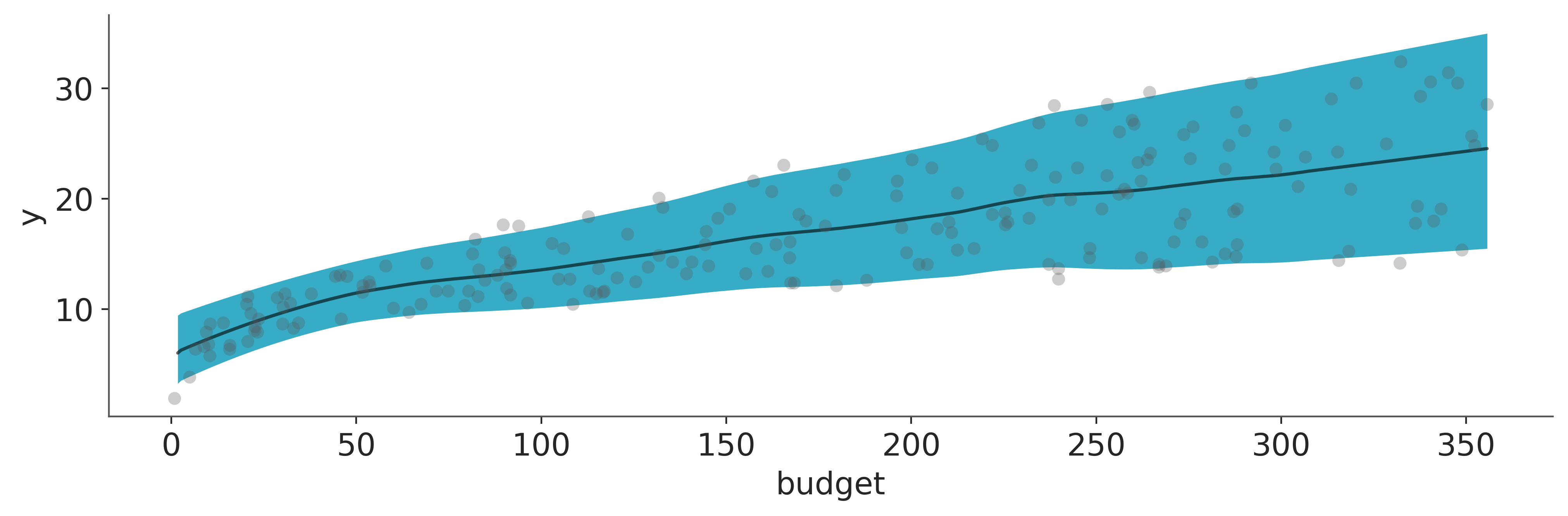
The fit looks good! In fact, we see that the mean and variance increase as a function of the budget.

Authors

• Authored by Juan Orduz in Feb, 2023

• Rerun by Osvaldo Martin in Mar, 2023

• Rerun by Osvaldo Martin in Nov, 2023

References

Watermark

%load_ext watermark
%watermark -n -u -v -iv -w -p pytensor

Last updated: Sat Nov 18 2023

Python implementation: CPython
Python version       : 3.11.5
IPython version      : 8.16.1

pytensor: 2.17.3

arviz     : 0.16.1
pandas    : 2.1.2
numpy     : 1.24.4
matplotlib: 3.8.0
pymc_bart : 0.5.3
pymc      : 5.9.2+10.g547bcb481

Watermark: 2.4.3