
PyMC 4.0 Release Announcement#
We, the PyMC core development team, are incredibly excited to announce the release of a major rewrite of PyMC3 (now called just PyMC): 4.0. Internally, we have already been using PyMC 4.0 almost exclusively for many months and found it to be very stable and better in every aspect. Every user should upgrade, as there are many exciting new updates that we will talk about in this and upcoming blog posts.
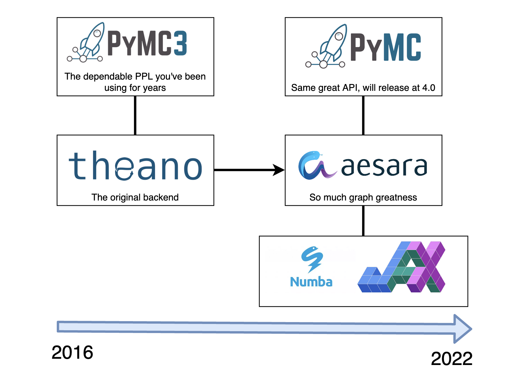
Graphic by Ravin Kumar#
Full API compatibility for model building#
To get the main question out of the way: Yes, you can just keep your existing PyMC modeling code without having to change anything (in most cases) and get all the improvements for free. The only thing most users will have to change is the import from import pymc3 as pm to import pymc as pm. For more information, see the quick migration guide. If you are using more advanced features of PyMC beyond the modeling API, you might have to change some things.
It’s now called PyMC instead of PyMC3#
First, the biggest news: PyMC3 has been renamed to PyMC. PyMC3 version 3.x will stay under the current name to not break production systems but future versions will use the PyMC name everywhere. While there were a few reasons for this, the main one is that PyMC3 4.0 looks quite confusing.
Theano → Aesara#
While evaluating other tensor libraries like TensorFlow and PyTorch as new backends we realized how amazing and unique Theano really was. It has a mature and hackable code base and a simple graph representation that allows easy graph manipulations, something that’s very useful for probabilistic programming languages. In addition, TensorFlow and PyTorch focus on a dynamic graph which is useful for some things, but for a probabilistic programming package, a static graph is actually much better, and Theano is the only library that provided this.
So, we went ahead and forked the Theano library and undertook a massive cleaning up of the code-base (this charge was led by Brandon Willard), removing swaths of old and obscure code, and restructuring the entire library to be more developer friendly.
This rewrite motivated renaming the package to Aesara (Theano’s daughter in Greek mythology). Quickly, a new developer team focused around improving aesara independent of PyMC.
What’s new in PyMC 4.0?#
Alright, let’s get to the good stuff. What makes PyMC 4.0 so awesome?

New JAX backend for faster sampling#
By far the most shiny new feature is the new JAX backend and the associated speed-ups.
How does it work? aesara provides a representation of the model logp graph in form of various aesara Ops (operators) which represent the computations to be be performed. For example exp(x + y) would be an Add Op with two input arguments x and y. The result of the Add Op is then inputted into an exp Op.
This computation graph doesn’t say anything about how we actually execute this graph, just what operations we want to perform. The functionality inherited from theano is to transpile this graph to C-code which would then get compiled, loaded into Python as a C-extension, and then could be executed very fast. But instead of transpiling the graph to C, aesara can now also target JAX.
This is very exciting, because JAX (through XLA) is capable of a whole bunch of low-level optimizations which lead to faster model evaluation, in addition to being able to run your PyMC model on the GPU.
Even more exciting is that this allows us to combine the JAX code that executes the PyMC model with a MCMC sampler also written in JAX. That way, the model evaluation and the sampler are one big JAX graph that gets optimized and executed without any Python call-overhead. We currently support a NUTS implementation provided by numpyro as well as blackjax.
Early experiments and benchmarks show impressive speed-ups. Here is a small example of how much faster this is on a fairly small and simple model: the hierarchical linear regression of the famous Radon example.
# Standard imports
import numpy as np
import arviz as az
import matplotlib.pyplot as plt
import seaborn as sns
import pandas as pd
RANDOM_SEED = 8927
rng = np.random.default_rng(RANDOM_SEED)
np.set_printoptions(2)

import os, sys
sys.stderr = open(os.devnull, "w")
In order to do side-by-side comparisons, let’s import both, the old PyMC3 and Theano as well as the new PyMC 4.0 and Aesara. For your own use-case, you will only need the new pymc packages of course.
# PyMC3 Imports
import pymc3 as pm3
import theano.tensor as tt
import theano

# PyMC 4.0 imports
import pymc as pm
import aesara.tensor as at
import aesara
Load in the radon dataset and preprocess it:
data = pd.read_csv(pm.get_data("radon.csv"))
county_names = data.county.unique()

data["log_radon"] = data["log_radon"].astype(theano.config.floatX)
county_idx, counties = pd.factorize(data.county)
coords = {"county": counties, "obs_id": np.arange(len(county_idx))}
Next, let’s define a hierarchical regression model inside of a function (see this blog post for a description of this model). Note that we provide pm, our PyMC library, as an argument here. This is a bit unusual but allows us to create this model in pymc3 or pymc 4.0, depending on which module we pass in. Here you can also see that most models that work in pymc3 also work in pymc 4.0 without any code change, you only need to change your imports.
def build_model(pm):
    with pm.Model(coords=coords) as hierarchical_model:
        # Intercepts, non-centered
        mu_a = pm.Normal("mu_a", mu=0.0, sigma=10)
        sigma_a = pm.HalfNormal("sigma_a", 1.0)
        a = pm.Normal("a", dims="county") * sigma_a + mu_a

        # Slopes, non-centered
        mu_b = pm.Normal("mu_b", mu=0.0, sigma=2.)
        sigma_b = pm.HalfNormal("sigma_b", 1.0)
        b = pm.Normal("b", dims="county") * sigma_b + mu_b

        eps = pm.HalfNormal("eps", 1.5)

        radon_est = a[county_idx] + b[county_idx] * data.floor.values

        radon_like = pm.Normal(
            "radon_like", mu=radon_est, sigma=eps, observed=data.log_radon,
            dims="obs_id"
        )

    return hierarchical_model
Create and sample model in pymc3, nothing special:
model_pymc3 = build_model(pm3)
%%time
with model_pymc3:
    idata_pymc3 = pm3.sample(target_accept=0.9, return_inferencedata=True)
CPU times: user 1.8 s, sys: 229 ms, total: 2.03 s
Wall time: 21.5 s
Create and sample model in pymc 4.0, also nothing special (but note that pm.sample() now returns and InferenceData object by default):
model_pymc4 = build_model(pm)
%%time
with model_pymc4:
    idata_pymc4 = pm.sample(target_accept=0.9)
CPU times: user 4.08 s, sys: 315 ms, total: 4.39 s
Wall time: 16.9 s
Now, lets use a JAX sampler instead. Here we use the one provided by numpyro. These samplers live in a different submodule sampling_jax but the plan is to integrate them into pymc.sample(backend="JAX").
import pymc.sampling_jax
%%time
with model_pymc4:
    idata = pm.sampling_jax.sample_numpyro_nuts(target_accept=0.9, progress_bar=False)
Compiling...
Compilation time =  0:00:00.648311
Sampling...
Sampling time =  0:00:04.195409
Transforming variables...
Transformation time =  0:00:00.025698
CPU times: user 7.51 s, sys: 108 ms, total: 7.62 s
Wall time: 5.01 s
That’s a 3x speed-up – for a single-line code change (although we’ve seen speed-ups much more impressive than that in the 20x range)! And this is just running things on the CPU, we can just as easily run this on the GPU where we saw even more impressive speed-ups (especially as we scale the data).
Again, for a more proper benchmark that also compares this to Stan, see this blog post.
Better integration into aesara#
The next feature we are excited about is a better integration of PyMC into aesara.
In PyMC3 3.x, the random variables (RVs) created by e.g. calling x = pm.Normal('x') were not truly theano Ops so they did not integrate as nicely with the rest of theano. This created a lot of issues, limitations, and complexities in the library.
Aesara now provides a proper RandomVariable Op which perfectly integrates with the rest of the other Ops.
This is a major change in 4.0 and lead to huge swaths of brittle code in PyMC3 get removed or greatly simplified. In many ways, this change is much more exciting than the different computational backends, but the effects are not quite as visible to the user. If you’re interested in how Aesara and PyMC interact in more detailed, check out the PyMC and Aesara tutorial.
There are a few cases, however, where you can see the benefits.
Faster posterior predictive sampling#
%%time

with model_pymc3:
    pm3.sample_posterior_predictive(idata_pymc3)
CPU times: user 1min 26s, sys: 2.48 s, total: 1min 28s
Wall time: 1min 29s
%%time

with model_pymc4:
    pm.sample_posterior_predictive(idata_pymc4)
CPU times: user 3.88 s, sys: 30.9 ms, total: 3.91 s
Wall time: 3.93 s
On this model, we get a speed-up of 22x!
The reason for this is that predictive sampling is now happening as part of the aesara graph. Before, we were walking through the random variables in Python which was not only slow, but also very error-prone, so a lot of dev time was spent fixing bugs and rewriting this complicated piece of code. In PyMC 4.0, all that complexity is gone.
Work with RVs just like with Tensors#
In PyMC3, RVs as returned by e.g. pm.Normal("x") behaved somewhat like a Tensor variable, but not quite. In PyMC 4.0, RVs are first-class Tensor variables that can be operated on much more freely.
with pm3.Model():
    x3 = pm3.Normal("x")

with pm.Model():
    x4 = pm.Normal("x")
type(x3)
pymc3.model.FreeRV
type(x4)
aesara.tensor.var.TensorVariable
Through the power of aeppl (a new low-level library that provides core building blocks for probabilistic programming languages on top of aesara), PyMC 4.0 allows you to do even more operations directly on the RV.
For example, we can just call aesara.tensor.clip() on a RV to truncate certain parameter ranges. Separately, calling .eval() on a RV samples a random draw from the RV, this is also new in PyMC 4.0 and makes things more consistent and allows easy interactions with RVs.
at.clip(x4, 0, np.inf).eval()
array(1.32)
trunc_norm = [at.clip(x4, 0, np.inf).eval() for _ in range(1000)]
sns.histplot(np.asarray(trunc_norm))
<AxesSubplot:ylabel='Count'>
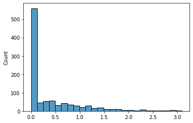
As you can see, negative values are clipped to be 0. And you can use this, just like any other transform, directly in your model.
But there are other things you can do as well, like stack() RVs, and then index into them with a binary RV.
with pm.Model():
    x = pm.Uniform("x", lower=-1, upper=0) # only negtive
    y = pm.Uniform("y", lower=0, upper=1) # only positive
    xy = at.stack([x, y]) # combined
    index = pm.Bernoulli("index", p=0.5) # index 0 or 1

    indexed_RV = xy[index] # binary index into stacked variable

for _ in range(5):
    print("Sampled value = {:.2f}".format(indexed_RV.eval()))
Sampled value = 0.82
Sampled value = 0.15
Sampled value = 0.31
Sampled value = -0.71
Sampled value = 0.00
As you can see, depending on whether index is 0 or 1 we either sample from the negative or positive uniform. This also supports fancy indexing, so you can manually create complicated mixture distribution using a Categorical like this:
with pm.Model():
    x = pm.Uniform("x", lower=-1, upper=0)
    y = pm.Uniform("y", lower=0, upper=1)
    z = pm.Uniform("z", lower=1, upper=2)
    xyz = at.stack([x, y, z])
    index = pm.Categorical("index", [.3, .3], shape=3)

    index_RV = xyz[index]

for _ in range(5):
    print("Sampled value = {}".format(index_RV.eval()))
Sampled value = [ 0.79 -0.28  0.79]
Sampled value = [0.37 0.37 0.37]
Sampled value = [-0.76  0.76  0.76]
Sampled value = [ 0.91 -0.2   0.91]
Sampled value = [0.78 0.78 0.78]
Better (and Dynamic) Shape Support#
Another big improvement in PyMC 4.0 is in how shapes are handled internally. Before, there was also a bunch of complicated and brittle Python code to handle shapes. Internally, we had a joke where we counted how many days had passed until we had discovered a new shape bug. But no more! Now, all shape handling is completely offloaded to aesara which handles this properly. As a side-effect, this better shape support also allows dynamic RV shapes, where the shape depends on another RV:
with pm.Model() as m:
    x = pm.Poisson('x', 2)
    z = pm.Normal('z', shape=x)

for _ in range(5):
    print("Value of z = {}".format(z.eval()))
Value of z = [-0.54 -0.24]
Value of z = [0.33]
Value of z = [-0.22 -0.67]
Value of z = []
Value of z = [ 2.01 -0.48]
As you can see, the shape of z changes with each draw according to the integer sampled by x.
Note, however, that this does not yet work for posterior inference (i.e. sampling). The reason is that the trace backend (arviz.InferenceData) as well as samplers in this case also must support changing dimensionality (like reversible-jump MCMC). There are plans to add this.
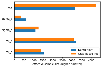
Better NUTS initialization#
We have also fixed an issue with the default NUTS warm-up which sometimes lead to the sampler getting stuck for a while. While fixing this issue, Adrian Seyboldt also came up with a new initialization method that uses the gradients to estimate a better mass-matrix. You can use this (still experimental) feature by calling pm.sample(init="jitter+adapt_diag_grad").
Let’s try this on the hierarchical regression model from above:
with model_pymc4:
    idata_pymc4_grad = pm.sample(init="jitter+adapt_diag_grad", target_accept=0.9)
The first thing to observe as that we did not get any divergences this time. Comparing the effective sample size of the default and grad-based initialization, we can also see that it leads to much better sampling for certain parameters:
pd.DataFrame({"Default init": az.summary(idata_pymc4, var_names=["~a", "~b"])["ess_bulk"],
              "Grad-based init": az.summary(idata_pymc4_grad, var_names=["~a", "~b"])["ess_bulk"]}).plot.barh()
plt.xlabel("effective sample size (higher is better)");
PyMC in the browser#
Did you know that you can run PyMC in the browser now too? This is possible with PyScript. Check out this blog post which has a small demo.
Installation#
Excited to try it out? Great! conda install -c conda-forge "pymc>=4" should get you going. For detailed instructions, see here.
New website#
We have also completely revamped our website, you can check it out at https://www.pymc.io. It’s not completely done yet so expect more improvements in the future. This effort was led by Oriol Abril.
A Look Towards the Future#
Samplers written in Aesara#
Above we described how with the new JAX backend we can run the model and the sampler as one big JAX graph, without any Python call-overhead. While this is already quite exciting, we can take this one step further. The setup we showed above takes the model logp graph (represented in aesara) and compiles it to JAX. The resulting JAX function can then be called from a sampler written in directly in JAX (i.e. numpyro or blackjax).
While lightning fast, this is suboptimal for two reasons:
For new backends, like
numba, we would need to write a new sampler implementation also innumba.While we get low-level optimizations from
JAXon the logp+sampler JAX-graph, we do not get any high-level optimizations, which is whataesarais great at, becauseaesaradoes not see the sampler.
With aehmc and aemcmc the aesara devs are developing a library of samplers written in aesara. That way, our model logp, consisting out of aesara Ops can then be combined with the sampler logic, now also consisting out of aesara Ops, and form one big aesara graph.
On that big graph containing model and sampler, aesara can the do high-level optimizations to get a more efficient graph representation. In a next step it can then compile it to whatever backend we want: JAX, numba, C, or whatever other backend we add in the future.
If you think this is interesting, definitely check out these packages and consider contributing, this is where the next round of innovation will come from!
Automatic model reparameterizations#
As mentioned in the beginning, aesara is a unique library in the PyData ecosystem as it is the only one that provides a static, mutable computation graph. Having direct access to this computation graph allows for many interesting features:
graph optimizations like
log(exp(x)) -> xsymbolic rewrites like
N(0, 1) + a->N(a, 1)
and aesara already implements many of these. While we don’t have proper benchmarks, we noticed major speed-ups of porting models from PyMC3 to 4.0, even without the JAX backend.
But these graph rewrites can become much more sophisticated. For example, a beta prior on a binomial likelihood can be replaced with its analytical solution directly by exploiting conjugacy.
Or a hierarchical model written in a centered parameterization can automatically be converted to its non-centered analog which often samples much more efficiently. These model reparameterizations can make a huge difference in how well a model samples. Unforutnately, these reparameterizations still require intimate knowledge of the math and a deep understanding of the posterior geometry, nothing a casual PyMC user would be familiar with. So with these graph rewrites we will be able to automatically reparameterize a PyMC model for you and find the configuration that samples most efficiently.
In sum, we believe PyMC 4.0 is the best version yet and pushes the state of the art in probabilistic programming. But it’s also stepping stone to many more innovations to come. Thanks for being a part of it.
Call to Action#
Want to help us build the future of probabilistic programming? It’s the perfect time to get involved. If you’re interested in:
user-friendly API → PyMC
documentation and examples → PyMC documentation
cutting-edge PyMC features (BART etc) → PyMC-experimental
low-level graph framework → aesara
Also, follow us on Twitter to stay up-to-date and join our MeetUp group for upcoming events. If you’re looking for consulting to solve your most challenging data science problems using PyMC, check out PyMC Labs – The Bayesian Consultancy.
Accolades#
While many people contributed to this effort, we would like to highlight the outstanding contributions of Brandon Willard, Ricardo Vieira, and Kaustubh Chaudhari who lead this gigantic effort.