


Bayes Factors and Marginal Likelihood#
import arviz as az
import numpy as np
import pymc as pm

from matplotlib import pyplot as plt
from matplotlib.ticker import FormatStrFormatter
from scipy.special import betaln
from scipy.stats import beta

print(f"Running on PyMC v{pm.__version__}")
Running on PyMC v5.0.0
az.style.use("arviz-darkgrid")
The “Bayesian way” to compare models is to compute the marginal likelihood of each model \(p(y \mid M_k)\), i.e. the probability of the observed data \(y\) given the \(M_k\) model. This quantity, the marginal likelihood, is just the normalizing constant of Bayes’ theorem. We can see this if we write Bayes’ theorem and make explicit the fact that all inferences are model-dependant.
where:
\(y\) is the data
\(\theta\) the parameters
\(M_k\) one model out of K competing models
Usually when doing inference we do not need to compute this normalizing constant, so in practice we often compute the posterior up to a constant factor, that is:
However, for model comparison and model averaging the marginal likelihood is an important quantity. Although, it’s not the only way to perform these tasks, you can read about model averaging and model selection using alternative methods here, there and elsewhere. Actually, these alternative methods are most often than not a better choice compared with using the marginal likelihood.
Bayesian model selection#
If our main objective is to choose only one model, the best one, from a set of models we can just choose the one with the largest \(p(y \mid M_k)\). This is totally fine if all models are assumed to have the same a priori probability. Otherwise, we have to take into account that not all models are equally likely a priori and compute:
Sometimes the main objective is not to just keep a single model but instead to compare models to determine which ones are more likely and by how much. This can be achieved using Bayes factors:
that is, the ratio between the marginal likelihood of two models. The larger the BF the better the model in the numerator (\(M_0\) in this example). To ease the interpretation of BFs Harold Jeffreys proposed a scale for interpretation of Bayes Factors with levels of support or strength. This is just a way to put numbers into words.
1-3: anecdotal
3-10: moderate
10-30: strong
30-100: very strong
\(>\) 100: extreme
Notice that if you get numbers below 1 then the support is for the model in the denominator, tables for those cases are also available. Of course, you can also just take the inverse of the values in the above table or take the inverse of the BF value and you will be OK.
It is very important to remember that these rules are just conventions, simple guides at best. Results should always be put into context of our problems and should be accompanied with enough details so others could evaluate by themselves if they agree with our conclusions. The evidence necessary to make a claim is not the same in particle physics, or a court, or to evacuate a town to prevent hundreds of deaths.
Bayesian model averaging#
Instead of choosing one single model from a set of candidate models, model averaging is about getting one meta-model by averaging the candidate models. The Bayesian version of this weights each model by its marginal posterior probability.
This is the optimal way to average models if the prior is correct and the correct model is one of the \(M_k\) models in our set. Otherwise, bayesian model averaging will asymptotically select the one single model in the set of compared models that is closest in Kullback-Leibler divergence.
Check this example as an alternative way to perform model averaging.
Some remarks#
Now we will briefly discuss some key facts about the marginal likelihood
The good
Occam Razor included: Models with more parameters have a larger penalization than models with fewer parameters. The intuitive reason is that the larger the number of parameters the more spread the prior with respect to the likelihood.
The bad
Computing the marginal likelihood is, generally, a hard task because it’s an integral of a highly variable function over a high dimensional parameter space. In general this integral needs to be solved numerically using more or less sophisticated methods.
The ugly
The marginal likelihood depends sensitively on the specified prior for the parameters in each model \(p(\theta_k \mid M_k)\).
Notice that the good and the ugly are related. Using the marginal likelihood to compare models is a good idea because a penalization for complex models is already included (thus preventing us from overfitting) and, at the same time, a change in the prior will affect the computations of the marginal likelihood. At first this sounds a little bit silly; we already know that priors affect computations (otherwise we could simply avoid them), but the point here is the word sensitively. We are talking about changes in the prior that will keep inference of \(\theta\) more or less the same, but could have a big impact in the value of the marginal likelihood.
Computing Bayes factors#
The marginal likelihood is generally not available in closed-form except for some restricted models. For this reason many methods have been devised to compute the marginal likelihood and the derived Bayes factors, some of these methods are so simple and naive that works very bad in practice. Most of the useful methods have been originally proposed in the field of Statistical Mechanics. This connection is explained because the marginal likelihood is analogous to a central quantity in statistical physics known as the partition function which in turn is closely related to another very important quantity the free-energy. Many of the connections between Statistical Mechanics and Bayesian inference are summarized here.
Using a hierarchical model#
Computation of Bayes factors can be framed as a hierarchical model, where the high-level parameter is an index assigned to each model and sampled from a categorical distribution. In other words, we perform inference for two (or more) competing models at the same time and we use a discrete dummy variable that jumps between models. How much time we spend sampling each model is proportional to \(p(M_k \mid y)\).
Some common problems when computing Bayes factors this way is that if one model is better than the other, by definition, we will spend more time sampling from it than from the other model. And this could lead to inaccuracies because we will be undersampling the less likely model. Another problem is that the values of the parameters get updated even when the parameters are not used to fit that model. That is, when model 0 is chosen, parameters in model 1 are updated but since they are not used to explain the data, they only get restricted by the prior. If the prior is too vague, it is possible that when we choose model 1, the parameter values are too far away from the previous accepted values and hence the step is rejected. Therefore we end up having a problem with sampling.
In case we find these problems, we can try to improve sampling by implementing two modifications to our model:
Ideally, we can get a better sampling of both models if they are visited equally, so we can adjust the prior for each model in such a way to favour the less favourable model and disfavour the most favourable one. This will not affect the computation of the Bayes factor because we have to include the priors in the computation.
Use pseudo priors, as suggested by Kruschke and others. The idea is simple: if the problem is that the parameters drift away unrestricted, when the model they belong to is not selected, then one solution is to try to restrict them artificially, but only when not used! You can find an example of using pseudo priors in a model used by Kruschke in his book and ported to Python/PyMC3.
If you want to learn more about this approach to the computation of the marginal likelihood see Chapter 12 of Doing Bayesian Data Analysis. This chapter also discuss how to use Bayes Factors as a Bayesian alternative to classical hypothesis testing.
Analytically#
For some models, like the beta-binomial model (AKA the coin-flipping model) we can compute the marginal likelihood analytically. If we write this model as:
the marginal likelihood will be:
where:
\(B\) is the beta function not to get confused with the \(Beta\) distribution
\(n\) is the number of trials
\(h\) is the number of success
Since we only care about the relative value of the marginal likelihood under two different models (for the same data), we can omit the binomial coefficient \(\binom {n}{h}\), thus we can write:
This expression has been coded in the following cell, but with a twist. We will be using the betaln function instead of the beta function, this is done to prevent underflow.
def beta_binom(prior, y):
    """
    Compute the marginal likelihood, analytically, for a beta-binomial model.

    prior : tuple
        tuple of alpha and beta parameter for the prior (beta distribution)
    y : array
        array with "1" and "0" corresponding to the success and fails respectively
    """
    alpha, beta = prior
    h = np.sum(y)
    n = len(y)
    p_y = np.exp(betaln(alpha + h, beta + n - h) - betaln(alpha, beta))
    return p_y
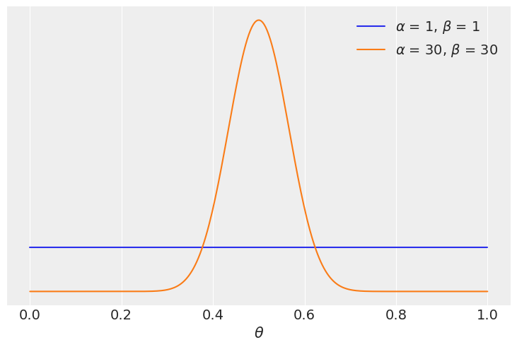
Our data for this example consist on 100 “flips of a coin” and the same number of observed “heads” and “tails”. We will compare two models one with a uniform prior and one with a more concentrated prior around \(\theta = 0.5\)
y = np.repeat([1, 0], [50, 50])  # 50 "heads" and 50 "tails"
priors = ((1, 1), (30, 30))
for a, b in priors:
    distri = beta(a, b)
    x = np.linspace(0, 1, 300)
    x_pdf = distri.pdf(x)
    plt.plot(x, x_pdf, label=rf"$\alpha$ = {a:d}, $\beta$ = {b:d}")
    plt.yticks([])
    plt.xlabel("$\\theta$")
    plt.legend()
The following cell returns the Bayes factor
BF = beta_binom(priors[1], y) / beta_binom(priors[0], y)
print(round(BF))
5
We see that the model with the more concentrated prior \(\text{beta}(30, 30)\) has \(\approx 5\) times more support than the model with the more extended prior \(\text{beta}(1, 1)\). Besides the exact numerical value this should not be surprising since the prior for the most favoured model is concentrated around \(\theta = 0.5\) and the data \(y\) has equal number of head and tails, consintent with a value of \(\theta\) around 0.5.
Sequential Monte Carlo#
The Sequential Monte Carlo sampler is a method that basically progresses by a series of successive annealed sequences from the prior to the posterior. A nice by-product of this process is that we get an estimation of the marginal likelihood. Actually for numerical reasons the returned value is the log marginal likelihood (this helps to avoid underflow).
models = []
idatas = []
for alpha, beta in priors:
    with pm.Model() as model:
        a = pm.Beta("a", alpha, beta)
        yl = pm.Bernoulli("yl", a, observed=y)
        idata = pm.sample_smc(random_seed=42)
        models.append(model)
        idatas.append(idata)
Initializing SMC sampler...
Sampling 4 chains in 4 jobs
/home/oriol/bin/miniconda3/envs/releases/lib/python3.10/site-packages/arviz/data/base.py:221: UserWarning: More chains (4) than draws (3). Passed array should have shape (chains, draws, *shape)
  warnings.warn(
Initializing SMC sampler...
Sampling 4 chains in 4 jobs
/home/oriol/bin/miniconda3/envs/releases/lib/python3.10/site-packages/arviz/data/base.py:221: UserWarning: More chains (4) than draws (1). Passed array should have shape (chains, draws, *shape)
  warnings.warn(
5.0
As we can see from the previous cell, SMC gives essentially the same answer as the analytical calculation!
Note: In the cell above we compute a difference (instead of a division) because we are on the log-scale, for the same reason we take the exponential before returning the result. Finally, the reason we compute the mean, is because we get one value log marginal likelihood value per chain.
The advantage of using SMC to compute the (log) marginal likelihood is that we can use it for a wider range of models as a closed-form expression is no longer needed. The cost we pay for this flexibility is a more expensive computation. Notice that SMC (with an independent Metropolis kernel as implemented in PyMC) is not as efficient or robust as gradient-based samplers like NUTS. As the dimensionality of the problem increases a more accurate estimation of the posterior and the marginal likelihood will require a larger number of draws, rank-plots can be of help to diagnose sampling problems with SMC.
Bayes factors and inference#
So far we have used Bayes factors to judge which model seems to be better at explaining the data, and we get that one of the models is \(\approx 5\) better than the other.
But what about the posterior we get from these models? How different they are?
az.summary(idatas[0], var_names="a", kind="stats").round(2)
| mean | sd | hdi_3% | hdi_97% | |
|---|---|---|---|---|
| a | 0.5 | 0.05 | 0.4 | 0.59 |
az.summary(idatas[1], var_names="a", kind="stats").round(2)
| mean | sd | hdi_3% | hdi_97% | |
|---|---|---|---|---|
| a | 0.5 | 0.04 | 0.42 | 0.57 |
We may argue that the results are pretty similar, we have the same mean value for \(\theta\), and a slightly wider posterior for model_0, as expected since this model has a wider prior. We can also check the posterior predictive distribution to see how similar they are.
ppc_0 = pm.sample_posterior_predictive(idatas[0], model=models[0]).posterior_predictive
ppc_1 = pm.sample_posterior_predictive(idatas[1], model=models[1]).posterior_predictive
Sampling: [yl]
Sampling: [yl]
_, ax = plt.subplots(figsize=(9, 6))

bins = np.linspace(0.2, 0.8, 8)
ax = az.plot_dist(
    ppc_0["yl"].mean("yl_dim_2"),
    label="model_0",
    kind="hist",
    hist_kwargs={"alpha": 0.5, "bins": bins},
)
ax = az.plot_dist(
    ppc_1["yl"].mean("yl_dim_2"),
    label="model_1",
    color="C1",
    kind="hist",
    hist_kwargs={"alpha": 0.5, "bins": bins},
    ax=ax,
)
ax.legend()
ax.set_xlabel("$\\theta$")
ax.xaxis.set_major_formatter(FormatStrFormatter("%0.1f"))
ax.set_yticks([]);
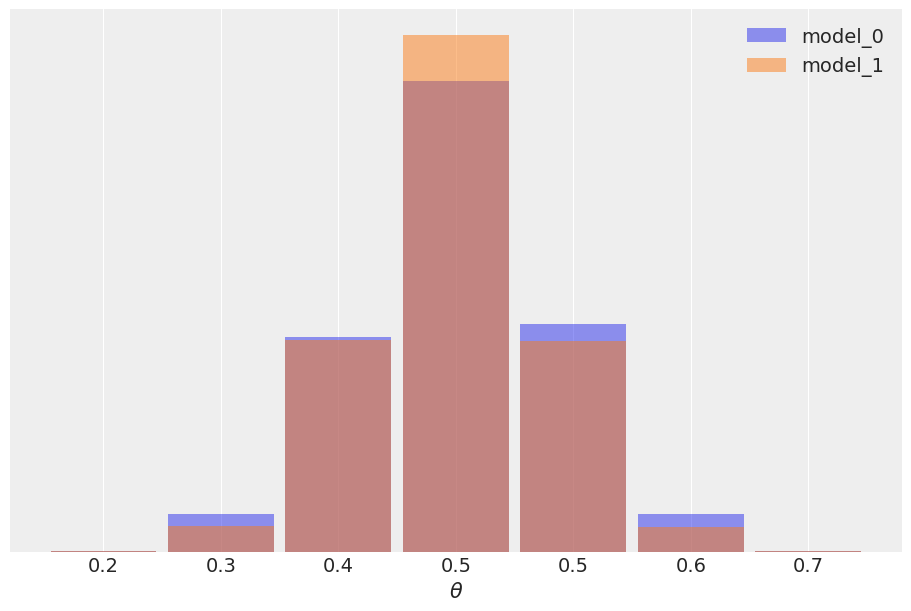
In this example the observed data \(y\) is more consistent with model_1 (because the prior is concentrated around the correct value of \(\theta\)) than model_0 (which assigns equal probability to every possible value of \(\theta\)), and this difference is captured by the Bayes factor. We could say Bayes factors are measuring which model, as a whole, is better, including details of the prior that may be irrelevant for parameter inference. In fact in this example we can also see that it is possible to have two different models, with different Bayes factors, but nevertheless get very similar predictions. The reason is that the data is informative enough to reduce the effect of the prior up to the point of inducing a very similar posterior. As predictions are computed from the posterior we also get very similar predictions. In most scenarios when comparing models what we really care is the predictive accuracy of the models, if two models have similar predictive accuracy we consider both models as similar. To estimate the predictive accuracy we can use tools like PSIS-LOO-CV (az.loo), WAIC (az.waic), or cross-validation.
Savage-Dickey Density Ratio#
For the previous examples we have compared two beta-binomial models, but sometimes what we want to do is to compare a null hypothesis H_0 (or null model) against an alternative one H_1. For example, to answer the question is this coin biased?, we could compare the value \(\theta = 0.5\) (representing no bias) against the result from a model were we let \(\theta\) to vary. For this kind of comparison the null-model is nested within the alternative, meaning the null is a particular value of the model we are building. In those cases computing the Bayes Factor is very easy and it does not require any special method, because the math works out conveniently so we just need to compare the prior and posterior evaluated at the null-value (for example \(\theta = 0.5\)), under the alternative model. We can see that is true from the following expression:
Which only holds when H_0 is a particular case of H_1.
Let’s do it with PyMC and ArviZ. We need just need to get posterior and prior samples for a model. Let’s try with beta-binomial model with uniform prior we previously saw.
with pm.Model() as model_uni:
    a = pm.Beta("a", 1, 1)
    yl = pm.Bernoulli("yl", a, observed=y)
    idata_uni = pm.sample(2000, random_seed=42)
    idata_uni.extend(pm.sample_prior_predictive(8000))
Auto-assigning NUTS sampler...
Initializing NUTS using jitter+adapt_diag...
Multiprocess sampling (4 chains in 4 jobs)
NUTS: [a]
Sampling 4 chains for 1_000 tune and 2_000 draw iterations (4_000 + 8_000 draws total) took 2 seconds.
Sampling: [a, yl]
And now we call ArviZ’s az.plot_bf function
az.plot_bf(idata_uni, var_name="a", ref_val=0.5);
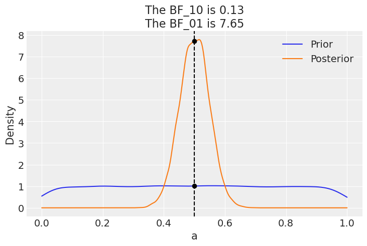
The plot shows one KDE for the prior (blue) and one for the posterior (orange). The two black dots show we evaluate both distribution as 0.5. We can see that the Bayes factor in favor of the null BF_01 is \(\approx 8\), which we can interpret as a moderate evidence in favor of the null (see the Jeffreys’ scale we discussed before).
As we already discussed Bayes factors are measuring which model, as a whole, is better at explaining the data. And this includes the prior, even if the prior has a relatively low impact on the posterior computation. We can also see this effect of the prior when comparing a second model against the null.
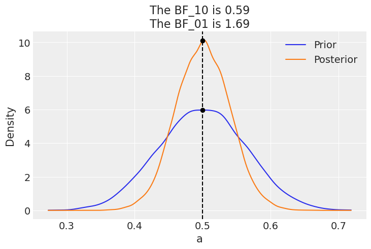
If instead our model would be a beta-binomial with prior beta(30, 30), the BF_01 would be lower (anecdotal on the Jeffreys’ scale). This is because under this model the value of \(\theta=0.5\) is much more likely a priori than for a uniform prior, and hence the posterior and prior will me much more similar. Namely there is not too much surprise about seeing the posterior concentrated around 0.5 after collecting data.
Let’s compute it to see for ourselves.
with pm.Model() as model_conc:
    a = pm.Beta("a", 30, 30)
    yl = pm.Bernoulli("yl", a, observed=y)
    idata_conc = pm.sample(2000, random_seed=42)
    idata_conc.extend(pm.sample_prior_predictive(8000))
Auto-assigning NUTS sampler...
Initializing NUTS using jitter+adapt_diag...
Multiprocess sampling (4 chains in 4 jobs)
NUTS: [a]
Sampling 4 chains for 1_000 tune and 2_000 draw iterations (4_000 + 8_000 draws total) took 2 seconds.
Sampling: [a, yl]
az.plot_bf(idata_conc, var_name="a", ref_val=0.5);
Authored by Osvaldo Martin in September, 2017 (pymc#2563)
Updated by Osvaldo Martin in August, 2018 (pymc#3124)
Updated by Osvaldo Martin in May, 2022 (pymc-examples#342)
Updated by Osvaldo Martin in Nov, 2022
Re-executed by Reshama Shaikh with PyMC v5 in Jan, 2023
References#
James M. Dickey and B. P. Lientz. The Weighted Likelihood Ratio, Sharp Hypotheses about Chances, the Order of a Markov Chain. The Annals of Mathematical Statistics, 41(1):214 – 226, 1970. doi:10.1214/aoms/1177697203.
Eric-Jan Wagenmakers, Tom Lodewyckx, Himanshu Kuriyal, and Raoul Grasman. Bayesian hypothesis testing for psychologists: a tutorial on the savage–dickey method. Cognitive Psychology, 60(3):158–189, 2010. URL: https://www.sciencedirect.com/science/article/pii/S0010028509000826, doi:https://doi.org/10.1016/j.cogpsych.2009.12.001.
Watermark#
%load_ext watermark
%watermark -n -u -v -iv -w -p pytensor
Last updated: Sun Jan 15 2023

Python implementation: CPython
Python version       : 3.10.8
IPython version      : 8.7.0

pytensor: 2.8.10

matplotlib: 3.6.2
numpy     : 1.24.0
pymc      : 5.0.0
arviz     : 0.14.0

Watermark: 2.3.1
License notice#
All the notebooks in this example gallery are provided under the MIT License which allows modification, and redistribution for any use provided the copyright and license notices are preserved.
Citing PyMC examples#
To cite this notebook, use the DOI provided by Zenodo for the pymc-examples repository.
Important
Many notebooks are adapted from other sources: blogs, books… In such cases you should cite the original source as well.
Also remember to cite the relevant libraries used by your code.
Here is an citation template in bibtex:
@incollection{citekey,
  author    = "<notebook authors, see above>",
  title     = "<notebook title>",
  editor    = "PyMC Team",
  booktitle = "PyMC examples",
  doi       = "10.5281/zenodo.5654871"
}
which once rendered could look like: