PyMC 6.0 & PyTensor 3.0: ecosystem updates

PyMC has been under steady development since the early 2010s. To mark the new major releases of PyMC 6.0 and PyTensor 3.0, we want to highlight the developments across the PyMC ecosystem (and its close cousin, the ArviZ ecosystem) that we’re most excited about.

The short version, before we dig in:

PyMC 6.0 is pip install-able with no extra system setup. The default computational backend is now Numba; C and JAX remain available on demand.

NUTS sampling is roughly 2x faster end-to-end, thanks to the new nutpie default sampler. pymc-extras adds Pathfinder and DADVI for variational inference.

The new pymc.dims module lets you write entire models against named dimensions. pymc-extras covers automatic marginalization of discrete latents and a high-level state-space API, and PyMC-BART covers Bayesian Additive Regression Trees.

pytensor.wrap_jax brings arbitrary JAX functions into PyMC models, and PyMC’s growing automatic logp derivation lets you build new distributions from existing ones.

ArviZ has reached 1.0 with a redesigned plotting library and xarray.DataTree-backed inference data. Kulprit brings projective variable selection, and PreliZ continues to grow as the prior-elicitation companion.

Performance

PyMC hasn’t always been a breeze to use. It’s written in Python, and its backend (Theano, and its successor PyTensor) had accrued some weight over the years.

A lot of effort was devoted to speeding up all stages of work: from import times, to model compilation and sampling runtime.

Numba is the new default backend

Historically, PyMC compiled model functions to C. In 6.0 we switch the default linker to Numba. For most CPU workloads Numba beats C, while being far easier to maintain and extend. It also unlocks a few things the old C path always struggled with:

• Native advanced indexing — the hierarchical-modelling staple that the C backend has always struggled with. Numba supports (almost) all cases natively and is noticeably faster.

• LAPACK bindings for linear algebra — cholesky, solve, eigh, and friends aren’t bottlenecked by Python.

• Fast scan — historically the slowest piece of the C backend, now far closer to looping in a low-level language (with autodiff). A big win for time-series and other recursive-structure models.

• Native sparse support — useful for spatial models (ICAR), state-space models, and INLA-style inference.

For GPU-based sampling, the JAX backend remains the recommended backend.

A knock-on win: PyMC is finally pip install-safe. The old C backend needed a system BLAS installation and a C compiler, both beyond pip’s reach. The first-time experience on a clean machine used to greet you with a prominent “PyTensor could not link to a BLAS installation” warning and degraded performance (or worse if a compiler couldn’t be detected). Conda/mamba was the only reliable path.

One-liner backend selection with backend=

You can pass backend= to every sampling and inference entry point (pm.sample, pm.sample_posterior_predictive, pm.fit, and so on).

Accepted values include "numba", "c", and "jax".

The default backend of pm.sample is "numba". You only need to pass it explicitly when picking something else.

Availability: Numba and C come with PyMC, though C needs both a compiler and a working BLAS installation at runtime to be usable. JAX has to be installed separately.

import matplotlib.pyplot as plt
import numpy as np
import pandas as pd

import pymc as pm

rng = np.random.default_rng(0)
y_obs = rng.normal(1.0, 0.5, size=50)

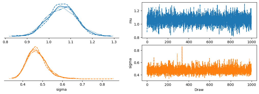
with pm.Model() as simple_model:
    mu = pm.Normal("mu")
    sigma = pm.HalfNormal("sigma")
    pm.Normal("y", mu=mu, sigma=sigma, observed=y_obs)

with simple_model:
    idata_numba = pm.sample(backend="numba", quiet=True)
    idata_jax = pm.sample(backend="jax", quiet=True)
    idata_c = pm.sample(backend="c", quiet=True)

All should arrive at the same place, if not at the same time.

pd.concat([
    pm.stats.summary(idata_numba, var_names=["mu"], kind="stats").rename({"mu": "mu (numba)"}),
    pm.stats.summary(idata_jax, var_names=["mu"], kind="stats").rename({"mu": "mu (jax)"}),
    pm.stats.summary(idata_c, var_names=["mu"], kind="stats").rename({"mu": "mu (c)"}),
])

	mean	sd	eti89_lb	eti89_ub
mu (numba)	1.1	0.067	0.95	1.2
mu (jax)	1.1	0.066	0.95	1.2
mu (c)	1.1	0.069	0.95	1.2

Inference

nutpie: the new default NUTS sampler

PyMC has historically latched onto Stan’s implementation of NUTS, borrowing its code almost line-by-line. It was time to contribute something back, and that something is nutpie.

You can easily install pymc and nutpie together as:

pip install pymc[nutpie]

Once installed, nutpie becomes the default NUTS in PyMC. Combined with the Numba backend, end-to-end sampling is roughly 2x faster than the old PyMC + C baseline on typical benchmarks, like the radon hierarchical model. Low-rank adaptation can push it to 4x. For the details, see Seyboldt, Carlson, & Carpenter (2026).

Three things set it apart from what we had before:

• Faster diagonal adaptation. nutpie often gets away with ~400 tuning draws where the old default conservatively used 1000, and after tuning it takes fewer leapfrog steps per draw.

• Low-rank mass-matrix adaptation. For posteriors with strongly correlated parameters, the diagonal mass matrix used by most HMC implementations is a poor fit. nutpie offers a low-rank extension of the diagonal that can dramatically reduce the number of gradient evaluations per effective draw on funnels, regressions with collinear predictors, and similar shapes.

• Native integration with Numba and JAX backends. No Python overhead.

An experimental normalizing-flow adaptation is also available for really difficult posteriors; see the nutpie docs.

If installed, nutpie (with diagonal adaptation) is selected automatically. You can manually switch between implementations using the nuts_sampler argument of pm.sample. Other options include "pymc", "numpyro", and "blackjax".

with simple_model:
    idata_nutpie = pm.sample(nuts_sampler="nutpie")

NUTS[nutpie]: [mu, sigma]

pm.stats.summary(idata_nutpie)

	mean	sd	eti89_lb	eti89_ub	ess_bulk	ess_tail	r_hat	mcse_mean	mcse_sd
mu	1.06	0.069	0.95	1.2	3573	2733	1.00	0.0012	0.00084
sigma	0.471	0.05	0.4	0.55	3791	2793	1.00	0.00084	0.00067

A classic nasty posterior: a simple linear regression where the covariate sits far from zero, making the intercept and slope strongly anti-correlated in the likelihood.

rng_corr = np.random.default_rng(1)
N = 200
x_far = rng_corr.normal(1000.0, 1.0, size=N)
y_far = 2.0 + 3.0 * x_far + rng_corr.normal(0.0, 1.0, size=N)

with pm.Model() as regression_far:
    a = pm.Normal("a", 0.0, 10)
    b = pm.Normal("b", 0.0, 10.0)
    sigma = pm.HalfNormal("sigma", 1.0)
    pm.Normal("y", mu=a + b * x_far, sigma=sigma, observed=y_far)

with regression_far:
    idata_diag = pm.sample(nuts={"adaptation": "diag"}, quiet=True)

pm.stats.summary(idata_diag, var_names=["a", "b"])

	mean	sd	eti89_lb	eti89_ub	ess_bulk	ess_tail	r_hat	mcse_mean	mcse_sd
a	-1	10.7	-17	17	305	371	1.01	0.61	0.41
b	3.002	0.0107	3	3	305	369	1.01	0.00061	0.00041

The low rank adaptation fares much better than the default diagonal mass matrix adaptation.

with regression_far:
    idata_lr = pm.sample(nuts={"adaptation": "low_rank"}, quiet=True)

pm.stats.summary(idata_lr, var_names=["a", "b"])

	mean	sd	eti89_lb	eti89_ub	ess_bulk	ess_tail	r_hat	mcse_mean	mcse_sd
a	-0.6	9.8	-16	15	6487	3271	1.00	0.12	0.084
b	3.0025	0.0098	3	3	6482	3142	1.00	0.00012	8.4e-05

Variational inference (pymc-extras): Pathfinder & DADVI

pymc-extras includes two modern Variational Inference solutions.

Pathfinder Pathfinder is a parallel quasi-Newton variational approximation: it runs L-BFGS from multiple starting points and combines the resulting trajectories using Pareto-smoothed importance sampling. It’s fast, parallelizable, and useful both as a NUTS warm-start and as a standalone approximation. See Zhang et al. (2022).

from pymc_extras import fit_pathfinder

with simple_model:
    idata_pf = fit_pathfinder(display_summary=False)

DADVI — Deterministic ADVI. Instead of stochastic optimization of the ELBO, it draws a fixed Monte Carlo sample upfront and hands the resulting deterministic objective to a second-order optimizer. Convergence is unambiguous (no more “is the ELBO done bouncing around?”), it works directly with off-the-shelf optimizers like L-BFGS, and linear-response covariance corrections fix the variance underestimation that mean-field ADVI is famous for. See Giordano, Ingram & Broderick (2024).

from pymc_extras.inference import fit_dadvi

with simple_model:
    idata_dadvi = fit_dadvi()

pd.concat([
    pm.stats.summary(idata_pf, var_names=["mu"], kind="stats").rename({"mu": "mu (pathfinder)"}),
    pm.stats.summary(idata_dadvi, var_names=["mu"], kind="stats").rename({"mu": "mu (dadvi)"}),
])

	mean	sd	eti89_lb	eti89_ub
mu (pathfinder)	1.1	0.069	0.95	1.2
mu (dadvi)	1.1	0.087	0.94	1.2

Modelling

A brief tour of four modelling additions: named-dimension models with pymc.dims, automatic marginalization of discrete latents, the state-space API, and PyMC-BART.

Named dims with pymc.dims

PyMC’s dims= argument has existed since 2020 to label the axes of model variables. The new pymc.dims module (backed by PyTensor’s XTensor) lets you write entire models against named dimensions, with automatic broadcasting, no more [:, None, :] gymnastics, and no more guessing which axis is which.

A compact example (adapted from the pymc.dims core notebook).

import pymc.dims as pmd

coords = {
    "participant": range(5),
    "trial": range(20),
    "item": range(3),
}
observed_response_np = np.ones((5, 20), dtype=int)

with pm.Model(coords=coords) as dmodel:
    observed_response = pmd.Data(
        "observed_response",
        observed_response_np,
        dims=("participant", "trial"),
    )

    participant_preference = pmd.ZeroSumNormal(
        "participant_preference",
        core_dims="item",
        dims=("participant", "item"),
    )
    time_effects = pmd.Normal("time_effects", dims=("item", "trial"))

    trial_preference = pmd.Deterministic(
        "trial_preference",
        participant_preference + time_effects,
    )

    response = pmd.Categorical(
        "response",
        p=pmd.math.softmax(trial_preference, dim="item"),
        core_dims="item",
        observed=observed_response,
    )

Note the absence of None-indexing to create new axes, right-aligning conventions or numerical axis arguments.

Also new: the Model.table() method renders a summary of every variable together with its expression and dimensions, a much more compact view than the good old Model.to_graphviz().

dmodel.table()

                 Variable  Expression                               Dimensions                           
─────────────────────────────────────────────────────────────────────────────────────────────────────────
      observed_response =  Data                                     participant[5] × trial[20]           
                                                                                                         
 participant_preference ~  ZeroSumNormal(<constant>, <constant>)    participant[5] × item[3]             
           time_effects ~  Normal(0, 1)                             item[3] × trial[20]                  
                                                                    Parameter count = 75                 
                                                                                                         
       trial_preference =  f(time_effects, participant_preference)  participant[5] × item[3] × trial[20] 
                                                                                                         
               response ~  Categorical(f(trial_preference))         participant[5] × trial[20]           

Automatic marginalization (pymc-extras)

Discrete latent variables are a pain to sample with gradient-based MCMC. Traditionally you’d have to sum them out by hand and rewrite your model as a marginal likelihood. pymc_extras.marginalize automates that process.

from pymc_extras import marginalize, recover_marginals

rng_mix = np.random.default_rng(2)
y_mix = rng_mix.normal(loc=np.tile([-2, 2], reps=50))
mix_coords = {"component": ["left", "right"], "obs": range(len(y_mix))}

with pm.Model(coords=mix_coords) as mix_model:
    w = pm.Dirichlet("w", a=np.ones(2))
    mu = pm.Normal("mu", mu=[-3.0, 3.0], dims="component")
    sigma = pm.HalfNormal("sigma", dims="component")
    z = pm.Categorical("z", p=w, dims="obs")
    pm.Normal("y", mu=mu[z], sigma=sigma[z], observed=y_mix, dims="obs")

with marginalize(mix_model, ["z"]) as marginal_model:
    idata_mix = pm.sample(quiet=True)

pm.stats.summary(idata_mix, var_names=["w", "mu"])

	mean	sd	eti89_lb	eti89_ub	ess_bulk	ess_tail	r_hat	mcse_mean	mcse_sd
w[0]	0.496	0.055	0.41	0.58	2474	2371	1.00	0.0011	0.00081
w[1]	0.504	0.055	0.42	0.59	2474	2371	1.00	0.0011	0.00081
mu[left]	-1.91	0.162	-2.2	-1.6	2266	2577	1.00	0.0034	0.0029
mu[right]	1.874	0.179	1.6	2.1	1973	1993	1.00	0.0041	0.0035

After sampling the marginalized model, you can still recover draws for the discrete latents with recover_marginals. The component assignments for each observation come back as proper posterior estimates.

with marginal_model:
    idata_mix = recover_marginals(idata_mix)

pm.stats.summary(idata_mix.isel(obs=slice(None, 6)), var_names=["z"], kind="stats")[["mean", "sd"]]

	mean	sd
z[0]	0.0047	0.069
z[1]	1	0.057
z[2]	0	0
z[3]	0.22	0.41
z[4]	0.38	0.48
z[5]	1	0.016

Statespace (pymc-extras)

pymc_extras.statespace offers Bayesian statespace models with an increasingly rich high-level API: BayesianETS, BayesianSARIMAX, BayesianVARMAX, plus a structural package for composing custom models out of level, trend, seasonal, and cyclical components.

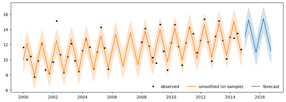
Here we fit a Holt–Winters ETS model (level + trend + additive quarterly seasonality) to a synthetic series generated from the same innovation-form process. Missing entries are imputed by the Kalman filter, and an 8-quarter forecast comes for free.

from pymc_extras.statespace.models import BayesianETS

rng = np.random.default_rng(3)
T, m = 60, 4
sigma_obs_true = 0.8
level, trend = 10.0, 0.05
seasonal = 2.0 * np.sin(2 * np.pi * np.arange(m) / m)
y_ts = np.array([
    level + trend * i + seasonal[i % m] + rng.normal(0, sigma_obs_true)
    for i in range(T)
])

dates = pd.date_range("2000-Q1", periods=T, freq="QS")
y_df = pd.DataFrame({"y": y_ts}, index=dates)
y_df.loc["2007-Q1":"2008-Q4", "y"] = np.nan  # Kalman filter will impute

ets = BayesianETS(
    order=("A", "A", "A"),
    endog_names=["y"],
    seasonal_periods=m,
    measurement_error=True,
    stationary_initialization=True,
)

                       Model Requirements                       
                                                                
  Variable           Shape   Constraints            Dimensions  
 ────────────────────────────────────────────────────────────── 
  initial_level      ()                                   None  
  initial_trend      ()                                   None  
  initial_seasonal   (4,)                    ('seasonal_lag',)  
  alpha              ()      0 < alpha < 1                None  
  beta               ()      0 < beta < 1                 None  
  gamma              ()      0 < gamma < 1                None  
  sigma_state        ()      Positive                     None  
  sigma_obs          ()      Positive                     None  
                                                                
 These parameters should be assigned priors inside a PyMC model 
    block before calling the build_statespace_graph method.     

with pm.Model(coords=ets.coords) as ets_model:
    pm.Normal("initial_level", mu=10, sigma=5)
    pm.Normal("initial_trend", mu=0, sigma=1)
    pm.ZeroSumNormal("initial_seasonal", sigma=2, dims="seasonal_lag")

    pm.Beta("alpha", 1, 1)
    pm.Beta("beta", 1, 1)
    pm.Beta("gamma", 1, 1)

    pm.Deterministic("sigma_state", pm.math.constant(np.array(0.0)))
    pm.HalfNormal("sigma_obs", 1)

    ets.build_statespace_graph(y_df)

    idata_ets = pm.sample(backend="jax", progressbar="combined")

ImputationWarning: Provided data contains missing values and will be automatically imputed as hidden states during Kalman filtering.
NUTS[nutpie]: [initial_level, initial_trend, initial_seasonal, alpha, beta, gamma, sigma_obs]

An 8-quarter forecast falls out of ets.forecast, and ets.sample_conditional_posterior fills in the imputed gap inside the training window. Structural decomposition and scenario analyses are similarly built in.

smoothed = ets.sample_conditional_posterior(idata_ets, progressbar=False)
forecast = ets.forecast(idata_ets, start=y_df.index[-1], periods=8, progressbar=False)

ImputationWarning: Provided data contains missing values and will be automatically imputed as hidden states during Kalman filtering.
Sampling: [filtered_posterior, filtered_posterior_observed, predicted_posterior, predicted_posterior_observed, smoothed_posterior, smoothed_posterior_observed]
ImputationWarning: Provided data contains missing values and will be automatically imputed as hidden states during Kalman filtering.
Sampling: [forecast_combined]

Plot the smoothed in-sample fit (orange) and the 8-quarter forecast (blue), with 89% credible bands.

sm = smoothed["smoothed_posterior_observed"].sel(observed_state="y")
fc = forecast["forecast_observed"].sel(observed_state="y")

fig, ax = plt.subplots(figsize=(12, 4))
ax.plot(y_df.index, y_df["y"], "k.", label="observed")
ax.plot(y_df.index, sm.mean(("chain", "draw")), "C1", label="smoothed (in-sample)")
ax.fill_between(
    y_df.index,
    sm.quantile(0.055, ("chain", "draw")),
    sm.quantile(0.945, ("chain", "draw")),
    color="C1",
    alpha=0.2,
)
ax.plot(fc.time, fc.mean(("chain", "draw")), "C0", label="forecast")
ax.fill_between(
    fc.time,
    fc.quantile(0.055, ("chain", "draw")),
    fc.quantile(0.945, ("chain", "draw")),
    color="C0",
    alpha=0.2,
)
ax.legend(loc="lower right", ncol=3, frameon=False);

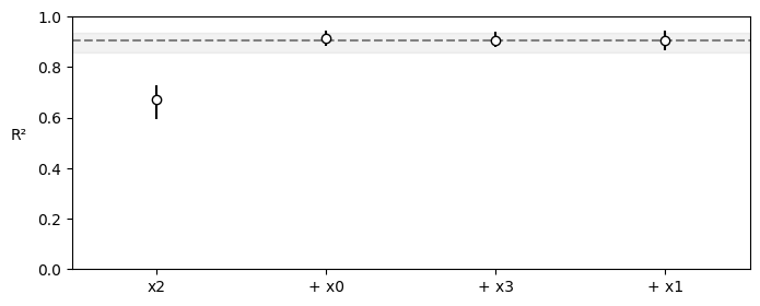
PyMC-BART

PyMC-BART brings Bayesian Additive Regression Trees to PyMC: a non-parametric prior on functions, expressed as an ensemble of decision trees.

Newer versions add plotting utilities (partial dependence, variable importance) and direct variable-importance integration with Kulprit (see next section). BART can then guide downstream variable selection on a parametric follow-up model. An experimental Rust tree sampler is also available.

import pandas as pd
import pymc_bart as pmb

rng_bart = np.random.default_rng(4)
n = 200
X_bart = pd.DataFrame(
    rng_bart.normal(size=(n, 4)),
    columns=["x0", "x1", "x2", "x3"],
)
# Only X_0 and X_2 actually drive the response
y_bart = np.sin(1.5 * X_bart["x0"]) + 0.7 * X_bart["x2"] ** 2 + rng_bart.normal(0, 0.3, n)

with pm.Model() as bart_model:
    mu = pmb.BART("mu", X_bart, y_bart, m=50)
    sigma = pm.HalfNormal("sigma", 1.0)
    pm.Normal("y", mu=mu, sigma=sigma, observed=y_bart)
    idata_bart = pm.sample(progressbar="combined")

Multiprocess sampling (4 chains in 4 jobs)
CompoundStep
>PGBART: [mu]
>NUTS: [sigma]
Sampling 4 chains for 1_000 tune and 1_000 draw iterations (4_000 + 4_000 draws total) took 53 seconds.
The rhat statistic is larger than 1.01 for some parameters. This indicates problems during sampling. See https://arxiv.org/abs/1903.08008 for details

# Variable importance — columns 0 and 2 should account for all cumulative R2.
vi = pmb.compute_variable_importance(idata_bart, bartrv=mu, X=X_bart)
pmb.plot_variable_importance(vi);

More building blocks

Two tools for when PyMC’s built-ins don’t quite fit: wrap_jax plugs arbitrary JAX functions into a model, and automatic logp derivation builds new distributions from existing ones.

Drop-in JAX with pytensor.wrap_jax

pytensor.wrap_jax lets you call any JAX-jittable function directly inside a PyMC model. That means the whole JAX ecosystem (Equinox neural networks, Diffrax ODE solvers, Optax optimizers) composes directly with your priors and likelihoods. Train a Bayesian neural network. Put a prior on the parameters of an ODE. Mix and match.

import jax.numpy as jnp
from pytensor import wrap_jax

@wrap_jax
def forward(x, a, b):
    return jnp.tanh(a * x + b)

rng = np.random.default_rng(5)
x_wj = rng.normal(size=100)
y_wj = np.tanh(0.8 * x_wj + 0.1) + rng.normal(0, 0.1, size=100)

with pm.Model() as wrap_jax_model:
    a = pm.Normal("a")
    b = pm.Normal("b")
    mu_wj = forward(x_wj, a, b)
    pm.Normal("y", mu=mu_wj, observed=y_wj)

    idata_wj = pm.sample(backend="jax", progressbar="combined")

pm.stats.summary(idata_wj)

NUTS[nutpie]: [a, b]

	mean	sd	eti89_lb	eti89_ub	ess_bulk	ess_tail	r_hat	mcse_mean	mcse_sd
b	0.13	0.152	-0.11	0.38	2229	2124	1.00	0.0032	0.0025
a	0.88	0.261	0.51	1.3	2159	2099	1.00	0.0058	0.0046

Sampling still runs through nutpie. backend="jax" just tells PyMC to compile the model through the JAX path, so the wrapped function stays native end-to-end.

Automatic probability & CustomDist

Most PPLs let you define models by chaining random variables and derive the log-density automatically. What’s less known is that PyMC can also derive log-densities for transformations of existing distributions: exponentiating, taking maxima, slicing. All without writing the math yourself.

Here we build a log-Student-T as exp of a Student-T, and ask PyMC for its log-density at 0.5

log_student_t = pm.math.exp(pm.StudentT.dist(nu=4, mu=0, sigma=1))

print(f"logp(LogStudentT, 0.5): {pm.logp(log_student_t, 0.5).eval():.4f}")

logp(LogStudentT, 0.5): -0.5713

The way to wire this into a model is with pm.CustomDist, which turns any dist-building function into a proper PyMC distribution:

def log_student_t_dist(nu, mu, sigma, size):
    return pm.math.exp(pm.StudentT.dist(nu=nu, mu=mu, sigma=sigma, size=size))


with pm.Model() as m:
    mu = pm.Normal("mu")
    sigma = pm.HalfNormal("sigma")
    y = pm.CustomDist("y", 4.0, mu, sigma, dist=log_student_t_dist, observed=0.5)

print(f"logp(y): {m.point_logps(round_vals=4)['y']}")

logp(y): -0.5713

Bayesian workflow

ArviZ 1.0

PyMC 6.0 is compatible with the new ArviZ 1.0. Most of the changes are invisible, the object returned by pm.sample still resembles the good old InferenceData, and the usual az.plot_* and az.summary calls keep working. For a full rundown, see the migration guide. A few changes worth knowing:

• InferenceData → xarray.DataTree. Arbitrary nesting is now allowed and any xarray-supported I/O format works. Existing netCDF/Zarr files keep loading.

• New plotting library. arviz-plots supports three backends (Matplotlib, Bokeh, Plotly) and returns a PlotCollection built on grammar-of-graphics ideas, with cleaner faceting and aesthetic mappings.

• New plots. The suite of built-in plots has grown notably around posterior-predictive checks. Browse them in the example gallery.

• New default credible interval has changed from 0.94 to 0.89, to remind everyone that no single number can rule us all. The default interval kind is now equal-tailed ("eti") rather than highest-density ("hdi"), and WAIC has been removed in favor of PSIS-LOO-CV.

Oh and plot_trace is now plot_trace_dist…

import arviz as az

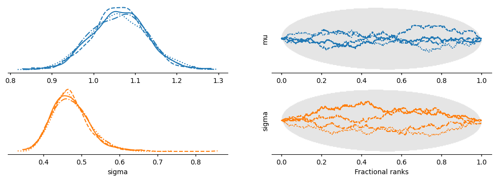
az.plot_trace_dist(idata_numba);

… although you may want to try plot_rank_dist instead.

az.plot_rank_dist(idata_numba);

PreliZ — prior elicitation

PreliZ helps with one of the trickiest parts of the Bayesian workflow: prior choice.

There’s a new Distributions Gallery to help get familiar with every family PreliZ supports.

Recent PreliZ work integrates PyMC distributions and pymc-extras Prior objects directly: maxent, matching, and plotting all accept them. from_pymc / from_prior convert them explicitly.

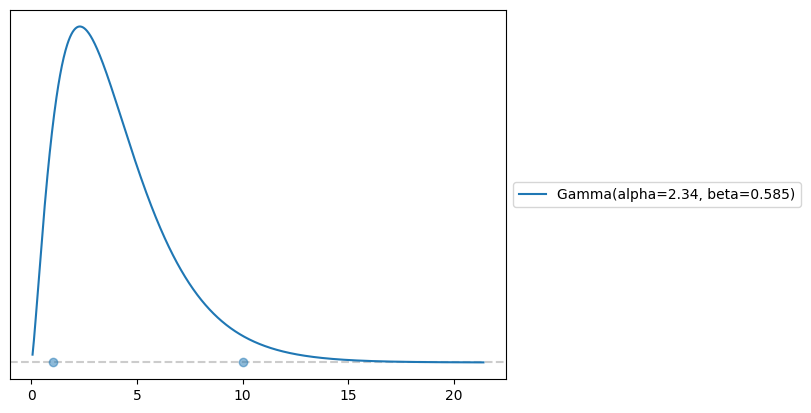
maxent is one of the package’s most useful tools: it picks the maximum-entropy distribution matching a target probability interval, a principled way to translate vague prior knowledge into a concrete prior. It also accepts any summary statistic (mean, variance, mode, …) as a fixed constraint:

import preliz as pz

# "Find a Gamma with mass 0.9 between 1 and 10 — and pin the mean to 4."
(prior, _fig) = pz.maxent(pz.Gamma(), lower=1, upper=10, mass=0.90, fixed_stat=("mean", 4))

with pm.Model() as m:
    x = prior.to_pymc("x")
    idata = pm.sample(quiet=True)
pm.stats.summary(idata)

	mean	sd	eti89_lb	eti89_ub	ess_bulk	ess_tail	r_hat	mcse_mean	mcse_sd
x	4	2.6	0.86	9	1196	1209	1.01	0.067	0.066

Kulprit — variable selection

Kulprit tackles a problem that shows up in almost every real study: you fit your best model with all the predictors you measured, but for interpretation or deployment you want a smaller one. Which predictors do you actually need?

Given a Bambi model with all candidates, Kulprit projects the full posterior onto smaller submodels using projective predictive inference. The projection keeps the uncertainty calibration of the original, and scales better than LOO-based comparison when the candidate count is large.

import bambi
import kulprit

# 4 candidate predictors; only x0 and x2 actually drive the response.
rng_k = np.random.default_rng(6)
n = 200
df_k = pd.DataFrame(rng_k.normal(size=(n, 4)), columns=["x0", "x1", "x2", "x3"])
df_k["y"] = 0.5 + 1.5 * df_k["x0"] + 0.8 * df_k["x2"] + rng_k.normal(0, 0.3, n)

full_model = bambi.Model("y ~ x0 + x1 + x2 + x3", df_k)
idata_full = full_model.fit(quiet=True)
pm.compute_log_likelihood(idata_full, model=full_model.backend.model, progressbar=False)

ppi = kulprit.ProjectionPredictive(full_model, idata_full)
ppi.project()
print(f"Selected: {ppi.select()}")

Selected: ['Intercept', 'x0', 'x2']

Thanks

Almost none of what we covered above came from a single person. Since the v5 and v2 releases of PyMC and PyTensor, each project has seen contributions from around 150 different individuals: bug fixes, documentation, new features, entire new packages. The surrounding libraries (ArviZ, nutpie, PyMC-BART, pymc-extras, PreliZ, Kulprit, Bambi) are maintained by a similarly broad and overlapping community.

Whether you’d like to contribute or just try things out, the PyMC Discourse is the easiest place to ask questions, share feedback, and discuss ideas. The GitHub repos are open for bug reports and pull requests. See you there.

Getting Started with PyMC